Download
1 / 32
320 likes | 575 Views
Disjoint Sets Data Structure (Chap. 21). A disjoint-set is a collection ={S 1 , S 2 ,…, S k } of distinct dynamic sets. Each set is identified by a member of the set, called representative . Disjoint set operations:

E N D
Disjoint Sets Data Structure (Chap. 21) • A disjoint-set is a collection ={S1, S2,…, Sk} of distinct dynamic sets. • Each set is identified by a member of the set, called representative. • Disjoint set operations: • MAKE-SET(x): create a new set with only x. assume x is not already in some other set. • UNION(x,y): combine the two sets containing x and y into one new set. A new representative is selected. • FIND-SET(x): return the representative of the set containing x.
Multiple Operations • Suppose multiple operations: • n: #MAKE-SET operations (executed at beginning). • m: #MAKE-SET, UNION, FIND-SET operations. • mn, #UNION operation is at most n-1.
An Application of Disjoint-Set • Determine the connected components of an undirected graph. • SAME-COMPONENT(u,v) • if FIND-SET(u)=FIND-SET(v) • thenreturn TRUE • elsereturn FALSE • CONNECTED-COMPONENTS(G) • for each vertex vV[G] • do MAKE-SET(v) • for each edge (u,v) E[G] • doif FIND-SET(u) FIND-SET(v) • then UNION(u,v)
Linked-List Implementation • Each set as a linked-list, with head and tail, and each node contains value, next node pointer and back-to-representative pointer. • Example: • MAKE-SET costs O(1): just create a single element list. • FIND-SET costs O(1): just return back-to-representative pointer.
c h f h f g e tail Linked-lists for two sets Set {c,h,e} head Set {f, g} g head tail UNION of two Sets c e head tail
UNION Implementation • A simple implementation: UNION(x,y) just appends x to the end of y, updates all back-to-representative pointers in x to the head of y. • Each UNION takes time linear in the x’s length. • Suppose n MAKE-SET(xi) operations (O(1) each) followed by n-1 UNION • UNION(x1, x2), O(1), • UNION(x2, x3), O(2), • ….. • UNION(xn-1, xn), O(n-1) • The UNIONs cost 1+2+…+n-1=(n2) • So 2n-1 operations cost (n2), average (n) each. • Not good!! How to solve it ???
Weighted-Union Heuristic • Instead appending x to y, appending the shorter list to the longer list. • Associated a length with each list, which indicates how many elements in the list. • Result: a sequence of m MAKE-SET, UNION, FIND-SET operations, n of which are MAKE-SET operations, the running time is O(m+nlg n). Why??? • Hints: Count the number of updates to back-to-representative pointer • for any x in a set of n elements. Consider that each time, the UNION • will at least double the length of united set, it will take at most lg n • UNIONS to unite n elements. So each x’s back-to-representative pointer • can be updated at most lg n times.
f c c f c c h e Disjoint-set Implementation: Forests • Rooted trees, each tree is a set, root is the representative. Each node points to its parent. Root points to itself. c c d d UNION h e Set {c,h,e} Set {f,d}
Straightforward Solution • Three operations • MAKE-SET(x): create a tree containing x. O(1) • FIND-SET(x): follow the chain of parent pointers until to the root. O(height of x’s tree) • UNION(x,y): let the root of one tree point to the root of the other. O(1) • It is possible that n-1 UNIONs results in a tree of height n-1. (just a linear chain of n nodes). • So n FIND-SET operations will cost O(n2).
Union by Rank & Path Compression • Union by Rank: Each node is associated with a rank, which is the upper bound on the height of the node (i.e., the height of subtree rooted at the node), then when UNION, let the root with smaller rank point to the root with larger rank. • Path Compression: used in FIND-SET(x) operation, make each node in the path from x to the root directly point to the root. Thus reduce the tree height.
Path Compression f f e c d e d c
Algorithm for Disjoint-Set Forest UNION(x,y) 1. LINK(FIND-SET(x),FIND-SET(y)) • MAKE-SET(x) • p[x]x • rank[x]0 • FIND-SET(x) • ifx p[x] • thenp[x] FIND-SET(p[x]) • returnp[x] • LINK(x,y) • ifrank[x]>rank[y] • thenp[y] x • else p[x] y • ifrank[x]=rank[y] • thenrank[y]++ Worst case running time for m MAKE-SET, UNION, FIND-SET operations is: O(m(n)) where (n)4. So nearly linear in m.
Analysis of Union by Rank with Path Compression(by amortized analysis) • Discuss the following: • A very quickly growing function and its very slowly growing inverse • Properties of Ranks • Proving time bound of O(m(n)) where (n) is a very slowly growing function.
A very quickly growing function and its inverse • For integers k0 and j 1, define Ak(j): • Ak(j)= j+1 if k=0 • Ak-1(j+1)(j) if k1 • Where Ak-10(j)=j, Ak-1(i)(j)= Ak-1(Ak-1(i-1)(j)) for i 1. • k is called the level of the function and • i in the above is called iterations. • Ak(j) strictly increase with both j and k. • Let us see how quick the increase is!!
Quickness of Function Ak(j)’s Increase • Lemma 21.2 (Page 510): • For any integer j, A1(j) =2j+1. • Proof: • By induction on i, prove A0i(j) =j+i. • So A1(j)= A0(j+1)(j) =j+(j+1)=2j+1. • Lemma 21.3 (Page 510): • For any integer j, A2(j) =2j+1(j+1)-1. • Proof: • By induction on i, prove A1i(j) =2i(j+1)-1 • A2(j)= A1(j+1)(j) = 2j+1(j+1)-1.
How Quick Ak(j) Increase • Let us see Ak(1): for k=0,1,2,3,4. • A0(1)=1+1=2 • A1(1)=2.1+1=3 • A2(1)=21+1(1+1)-1=7 • A3(1)=A2(1+1)(1)=A2(2)(1)=A2(A2(1))=A2(7)=27+1(7+1)-1=28.8-1=2047 • A4(1)=A32(1)=A3(A3(1)) =A3(2047)=A2(2048)(2047) >> A2(2047) =22048.2048-1 >22048 =(24)512 =(16)512 • >>1080. (estimated number of atoms in universe)
Inverse of Ak(n):(n) • (n)=min{k: Ak(1) n} (so, A(n)(1) n ) • (n)= 0 for 0 n 2 • 1 n =3 • 2 for 4 n 7 • 3 for 8 n 2047 • 4 for 2048 n A4(1). • Extremely slow increasing function. • (n) 4 for all practical purposes.
O(m(n)) bound: Property of Ranks • Lemma 21.4 (page 511): • For all nodes x, rank[x] rank[p[x]], with strict inequality if xp[x]. • Corollary 21.5 (page 511): • As we follow the path from any node to the root, the node ranks strictly increase. • Lemma 21.6 (page 512): • Every node had rank at most n-1. • Proof: rank begins with 0, increase possibly with only LINK operations, which is at most n-1 time. • In fact, at most log(n).
O(m(n)) bound proof • Using amortized analysis (Chap. 17) • Using LINK instead UNION (every UNION is done by two FIND-SETs and one LINK) • Lemma 21.7 (page 512): • Suppose converting a sequence S' of m'MAKE-SET, UNION, and FIND-SET operations into a sequence S of m MAKE-SET, LINK, FIND-SET by turning UNION to two FIND-SETs and one LINK, then if S runs in O(m(n)), then S' runs in O(m'(n)). • Proof: because of m' m 3m' , thus m=O(m').
Potential Function • For each node x, assign a potential function q(x) after q operations. • Then potential for entire forest, q=xq(x) • 0=0 at the beginning. • q will never be negative. • q(x)= (n)rank[x] if x is a root or rank[x]=0. • (n)-level(x)rank[x]-iter(x) otherwise.
level(x) and iter(x) • level(x)=max{k: rank[p[x]]Ak(rank[x])} • 0 Level(x)<(n), since • rank[p[x]]rank[x]+1=A0(rank[x]) and • A(n) (rank[x]) A(n) (1) n > rank[p[x]]. • iter(x)=max{i: rank[p[x]]Alevel(x)(i)(rank[x])} • 1 iter(x) rank[x], since • rank[p[x]]Alevel(x)(rank[x])=Alevel(x)(1)(rank[x]) and • Alevel(x)(rank[x]+1)(rank[x])=Alevel(x)+1(rank[x])>rank[p[x]].
Relations among rank[p[x]], level(x) and iter(x) • Since rank[p[x]] monotonically increase over time, in order for iter(x) to decrease, level(x) must increase. • Or say another way, as long as level(x) remains unchanged, iter(x) must either increase or remains unchanged.
Properties for Potential Function q(x) • Lemma 21.8 (page 514): • For every node x, and for all q, 0 q(x) (n)rank[x] • Proof: • if x is a root or rank[x]=0, then correct by definition. • Suppose x is not a root and rank[x]>0, • q(x)= [(n)-level(x)]rank[x]-iter(x) ((n)-((n)-1)) rank[x]-rank[x] =rank[x]-rank[x]=0. • q(x)= [(n)-level(x)]rank[x]-iter(x) [(n)-0]rank[x]-1= (n)rank[x]-1<(n)rank[x]
Potential Changes of Operations • Lemma 21.9 (page 515): • Let x be a node that is not a root, and suppose qth operation is either LINK or FIND-SET. Then after the qth operation, q(x) q-1(x). Moreover, if rank[x] 1 and either level[x] or iter(x) changes due to the qth operation, then q(x) q-1(x)-1. • Proof: • x not root rank[x] not change • n not change (n) not change. • If rank[x]=0, then q(x) =q-1(x)=0. suppose rank[x]>0. • If level(x) not change, • If iter(x) not change, q(x) =q-1(x), since all keep same • If iter(x) increase, then at lease by 1, q(x) will decrease at least 1. • If level(x) increases (at least by 1), then ((n)-level(x))rank[x] drops at least by rank[x] . • Suppose iter(x) drops, then, the drop is at most rank[x]-1. so q(x) will drop at least rank[x]-(rank[x]-1)=1. Thus q(x) q-1(x)-1.
Amortized Costs of Operations • Lemma 21.10 (page 515): • The amortized cost of each MAKE-SET operation is O(1). • Proof: create a single node x with rank 0, so q(x) =0. no other change to the forest, so q= q-1. The left is the actual cost, which is O(1).
Amortized Costs of Operations (cont.) • Lemma 21.11 (page 515): • The amortized cost of each LINK operation is O((n)). • Proof: (LINK(x,y) makes y the parent of x). • Actual cost for LINK operation is O(1). • Considering potential change: • Three kinds of nodes: x, y, and the old children of y. • By Lemma 21.9, the potential of y’s old children not increase. • For x (changed to non-root from a root), q(x)= [(n)-level(x)]rank[x]-iter(x) [(n)-0]rank[x]-1= (n)rank[x]-1<(n)rank[x]=q-1(x). • For y, rank[y] may stay same or increase by 1, so q(y)=(n)rank[y]=q-1(y) or q-1(y)+(n). • Thus the potential increase due to the LINK operation is at most (n). • Thus the amortized cost is O(1)+O((n))=O((n))
Amortized Costs of Operations (cont.) • Lemma 21.12 (page 516): • The amortized cost of each FIND-SET operation is O((n)). • Proof: suppose there are s nodes in the find path. • The actual cost of FIND-SET is O(s). • Root’s potential does not change and no other node’s potential increases (by Lemma 21.9). • At least max(0,s-((n)+2)) nodes on the find path have their potential decrease by at least 1. • Thus the amortized cost is at most O(s)-(s-((n)+2)) =O((n)).
Proof of Lemma 21.12 (cont.) • Proof that at lease max(0,s-((n)+2)) nodes on the find path have their potential decrease by at least 1. • Let x be a node on the find path: • rank[x]>0, • followed somewhere by y that is not a root, • and level(y)=level(x) just before FIND-SET. • At most (n)+2 nodes do not satisfy: 1th node, root node, the last node w for which level(w)=0,1,…, (n)-1. • Thus at least max(0,s-((n)+2)) nodes satisfy. • Let us fix x, show x’s potential decreases by at least 1.
Proof of Lemma 21.12 (cont.) • Let k=level(x)=level(y), Just prior to path compression caused by FIND-SET, we have • rank[p[x]]Ak(iter(x))(rank[x]) (by iter(x)’s def.) • rank[p[y]]Ak(rank[y]) (by level(y)’s def.) • rank[y] rank[p[x]] (since y follows x somewhere). • Let i=iter(x) before path compression, we have • rank[p[y]]Ak(rank[y]) Ak(rank[p[x]]) (since Ak(j) is strictly increasing) Ak(Ak(iter(x))(rank[x])) =Ak(i+1)(rank[x]) • After path compression, rank[p[x]]=rank[p[y]], which not decrease, and rank[x] not change, so rank[p[x]]Ak(i+1)(rank[x]). • Which means that either iter(x) increases (to at least i+1), or level(x) to increase. Thus by Lemma 21.9, q(x) q-1(x)-1. that is x’s potential decreases by at least 1. • As a result, we prove the lemma 21.12.
Upper bound for Disjoint-sets • Theorem 21.13 (page 517): • A sequence of m MAKE-SET, UNION, FIND-SET operations, n of which are MAKE-SET operations, can be performed on a disjoint-set forest with union by rank and path compression in worst cast time O(m(n)).
Summary • Disjoint set • Three operations • Different implementations and different costs • Forest implementation: • Union by rank and path compression • Properties: rank, level, iter. • Amortized analysis of the operations: • Potential function. • Ak(j) funcion: • Ak(j)= j+1 if k=0 • Ak-1(j+1)(j) if k1 • Where Ak-10(j)=j, Ak-1(i)(j)= Ak-1(Ak-1(i-1)(j)) for i 1. • k is called the level of the function and • i in the above is called iterations. • (n)=min{k: Ak(1) n}
A typical example using Disjoint Set • Kruskal's algorithm (Minimum Spanning Tree) • sort the edges of G in increasing order by length • keep a subgraph S of G, initially empty • for each edge e in sorted order • if the endpoints of e are disconnected in S • add e to S • return S • Note: greedy algorithm • Analysis: The testing whether two endpoints are disconnected • looks like it should be slow (linear time per iteration, or O(mn) total). • in fact, constant time.