Download
1 / 40
400 likes | 643 Views
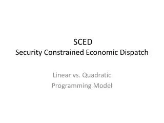
Security Constrained Economic Dispatch. Resmi Surendran. Outline. Overview of the SCED Texas two step SCED optimization. Security Constrained Economic Dispatch.

E N D
Security Constrained Economic Dispatch Resmi Surendran
Outline • Overview of the SCED • Texas two step • SCED optimization
Security Constrained Economic Dispatch • SCED evaluates Energy Offer Curves to produce a least cost dispatch of On-Line Resources while respecting transmission and generation constraints. • Manages the transmission system reliability and security • Operates within the physical constraints of the system • Meets the power balance while maintaining system reliability at minimum cost • SCED is executed: • Every 5 minutes (at a minimum) • May be initiated more often by an ERCOT operator or other ERCOT systems
Components Different components of the RT system
SCED – Input /Output • SCED Inputs: • Energy Offer Curves • Output Schedule • Mitigated offer cap /floor curves • Telemetry • Resource limits • Network constraints flow and limit • Competitive constraints • SCED outputs: • LMPs • Resource-Specific Base Points
Energy Offer Curve $/MWH Real Price Curve Piecewise Linear (ERCOT) Stepwise Approximation MW Pmin Pmax
Proxy Energy Offer Curve: Resource without Full Offer Range QSE-submitted Energy Offer Curves are extended from 0MW to infinity;
Proxy Energy Offer Curve: Resource with Output Schedule Proxy energy curves are created for resources with Output Schedules and no Incremental/Decremental Offer Curves;
Proxy Energy Offer Curve: Wind Powered Resource without Offer Proxy energy curves are also created for wind-powered resources that have not submitted Energy Offer Curves.
Resource Limits Resource Limits calculated by RLC is used in SCED and LFC
Constraints • Generated by doing contingency analysis based on State Estimator results • Removes constraints that are resolved by SPS and RAPs • Constraints are passed to SCED only if approved by operator in Transmission Constraint Manager (TCM) • Operator removes constraints that for which there are no Market solution or which has temporary ction plan developed due to some outages • Both competitive and non-competitive constraints are passed to SCED from TCM.
SCED – The Texas Two Step • SCED optimization executes twice each cycle • To ensure competition and reduce Market Power • Constraints are classified beforehand • Competitive • Non-Competitive • Step 1 • Uses the Energy Offer Curves for all On-Line Generation Resources • Observes the limits of the Competitive Constraints only • Determines “Reference LMPs“ • Step 2 • Observes limits of all Competitive and Non-Competitive Constraints • The Energy Offer Curve for any on-line Resource is capped at the greater of the Reference LMP from Step 1 or the Mitigated Offer Cap. • The Energy Offer Curve for any on-line Resource is bounded at the lesser of the Reference LMP from Step 1 or the Mitigated Offer Floor.
Two-Step SCED-Step 1: • Uses the Energy Offer Curves for all On-Line Generation Resources • Submitted or created by ERCOT • Only observes the limits of the Competitive Constraints only • Determines “Reference LMPs“
Data Processing between SCED Step 1 and Step 2 (1)Cap the Energy Offer Curves at the greater of the Reference LMP at the Resource Node or the Mitigated Offer Cap curve (2) Bound it at the lesser of the Reference LMP at the Resource Node or the Mitigated Offer Floor.
Two-Step SCED-Step 2: • Uses the capped and bounded Energy Offer curve • Observes limits of all Competitive and Non-Competitive Constraints • Creates LMPs, Base Points, Shadow Prices for the constraints etc
SCED - Two-Step Outputs SCED Two-step Reference Locational Marginal Prices (LMPs) Step 1 (only Competitive Constraints) Capped and bounded energy offer curves Base Points & final LMPs Settlement Point Prices (SPP) Initial data processing Data processing between step 1 and step 2 Step 2 (both Competitive and Non-Competitive Constraints)
SCEDObjective Minimize Cost of dispatching generation integral (offer cost * MW dispatched) + Penalty for violating Power Balance constraint sum (Penalty cost * violation amount) + Penalty for violating transmission constraint sum (Penalty cost * violation amount)
SCEDConstraints • Power Balance Constraint sum (Base Point) + under gen slack – over gen slack = Generation to be dispatched • Transmission constraint sum( Shift Factor * Base Point) – violation slack ≤ limit • Ramp Limit constraint LDL ≤ Base Point ≤ HDL
PowerBalancePenaltyCurve The SCED under generation Power Balance Penalty Curve will be capped at 2251 until the HCAP becomes 3000.
PowerBalancePenalty • Power Balance Penalty is the maximum cost paid for one addition/less MW of generation to meet the load. i.e. It caps the energy component of the LMP. • It sets the energy price in case of scarcity • ERCOT doesn’t have price caps • SWCAP caps the offers and not the prices • i.e. with SWCAP at $180 and the Power Balance Penalty curve up to 3000 the system wide prices could go up to 3000 and higher than 3000 in specific areas if there is congestion
Transmission Constraint Maximum Shadow Prices • Default maximum Shadow Price are assigned to monitored elements based on voltage level. These could be assigned higher or lower values based on operational experience. • Base Case: $5,000/MW • Generic constraints : $5,000/MW • Post Contingency • 345 kV: $4,500/MW • 138 kV: $3,500/MW • 69 kV: $2,800/MW
Shadow Price Shadow Price of a constraint is the increase in the objective when the constraint limit is reduced by 1 MW Maximum Shadow Price is set as the coefficient of the slack variable corresponding to the constraint in the SCED objective function. i.e. it is the maximum allowed increase in production cost for resolving 1MW of the constraint. Objective = Min ( Cost of generation dispatch + Sum ( Maximum Shadow Price * Slack variable) LMP at any electrical bus is Energy Component = Shadow price of Power Balance constraint + Congestion Component = - sum ( Shift Factor * Shadow Price for the constraint )
LMPduringCongestion Resource moved down for congestion
LMPduringCongestion Resource moved up for congestion
SCED Mathematical Formulation in Theory Minimize Sumseg&unit { Ccost = ½ ∙ aslope ∙ P2unit + Punit∙ bconst + cmincost } Subject to: sumseg&unit { Punit } = Pload - Power balance sumseg&unit { SFunit/line ∙ Punit } ≤ Limitline - Transmission limits Pmin ≤ sumseg{Punit} ≤ Pmax - Unit limits
Optimality Conditions Lagrange Function: L = sumseg&unit { ½ ∙ aslope ∙ P2unit + Punit∙ bconst + cmincost } + λ ∙ (Pload – sumseg&unit { Punit }) + sumline {µline∙ (Limitline – sumseg&unit { SFunit/line ∙ Punit } ) } Optimality Conditions: (1)d L /dPunit = aslope ∙ Punit + bconst - λ - sumline {µline ∙ SFunit/line } = 0 (2)sumseg&unit { Punit } = Pload - Power balance (3)sumseg&unit { SFunit/line ∙ Punit } + Fslack = Limitline - Transmission limits (4)µline ∙ Fslack = 0 - complementary slackness (5)Pmin ≤ sumseg {Punit }≤ Pmax ; (6)Fslack ≥ 0
SCED Objective Objective = Min { Cost of generation dispatch + Sum ( Max Shadow Price * Slack variable)} Generation dispatch cost + Slack Variable Slack Variable Max Shadow Price + Slack Variable Max Shadow Price
SCED Constraints Power Balance Constraints: ) ( Transmission Network Constraints: ( ) Resource Constraints: Ramp Rate Constraints (HDL, LDL):
Caculate LMP at each bus at target time t • LMPs are used to calculate Settlement Point Prices.
Calculate Settlement Point Price (SPP) Types of Settlement Points: – Resource Nodes – Load Zones – Hubs
Resource Node SPP Resource Nodes • A Resource Node is an Electrical Bus where a Generation Resource’s measured output is settled. The Real-Time Settlement Point Price for a Resource Node Settlement Point is a Base-Point time-weighted average of the Real-Time LMPs. RTSPP = Where the Resource Node weighting factor is: y - A SCED interval in the 15-minute Settlement Interval. r - A Resource at the Resource Node.
Load Zone • Load Zones • A Load Zone is a group of Electrical Buses, each with a load, which are assigned to the same zone for settlement purposes. • • Three types of Load Zones • – Competitive Load Zones • ◦ Four congestion zones in effect during the 2003 ERCOT market • – Non-Opt in Entity (NOIE) Load Zones • – DC Tie Load Zones
Load Zone SPP • A, B, C, and D are all electrical buses within Load Zone • Dollar amounts represent LMPs Total Load = 10 MW Percentage of load at each bus A: 2 / 10 = 20% B: 2 / 10 = 20% C: 1 / 10 = 10% D: 5 / 10 = 50% $4 2 MW $1 2 MW $10 5 MW Load-weighted avg. of LMPs at all buses = (20% * LMPbus A ) + (20% * LMPbus B) + (10% * LMPbus C) + (50% * LMPbus D) = (20% * $4 ) + (20% * $1 ) + (10% * $20 ) + (50% * $10 ) = $0.80 + $0.20 + $2.00 + $5.00 = $8.00 $20 1 MW Calculation of Load Zone Settlement Point Prices – Load-weighted average of LMPs at all buses assigned to that Zone – In Real-Time, LMPs will also be time-weighted.
HUBs Hubs • Hubs are defined by the Protocols – Hubs consist of Hub Buses – Hub Buses consist of one or more electrical buses within a single substation. • Hubs are only used for trading purposes
HUB SPP • The blue boxes represent Hub Buses within the Hub • The orange rectangles represent Electrical buses within the Hub Buses First, determine simple averages for all Hub Buses: A and D only have one bus: LMPs For Hub Bus A = $5 For Hub Bus D = $20 LMP = $5 LMP = $8 LMP = $12 LMP = $4 LMP = $20 LMP = $9 LMP = $2 LMPs Hub Bus B = ($8 + $12) / 2 = $10 Hub Bus C = ($4 + $9 + $2) / 3 = $5 Hub Settlement Point Price = (LMPA + LMPB + LMPC + LMPD) / 4 = ($5 + $10 + $5 + $20) / 4 = $40 / 4 = $10 Calculation of Hub Settlement Point Prices – Simple average of Hub Bus LMPs – Hub Bus LMP is the simple average of LMPs at Electrical Buses within the Hub Bus. – In Real-Time, LMPs will also be time-weighted.