High P T Hadron Collider Physics

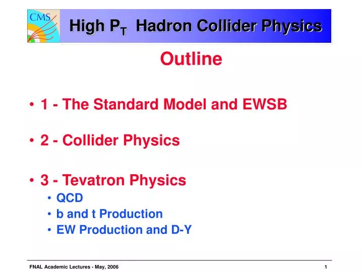
1. High PT Hadron Collider Physics • Outline • 1 - The Standard Model and EWSB • 2 - Collider Physics • 3 - Tevatron Physics • QCD • b and t Production • EW Production and D-Y

2. Backup Text

3. Units

4. Tools Needed (will use both during lecture demonstrations) ( Google them all – also Ghostview and Acrobat reader )

5. COMPHEP – Models and Particles Can edit the couplings – e.g. ggH Use SM Feynman gauge Watch for LOCK

6. COMPHEP - Process 1-> 2,3 1-> 2,3,4 1,2 ->3,4 1,2 ->3,4,5 1,2-> 3,4,5,6 (slow) *x options No 2 -> 1

7. COMPHEP –Simpson, BR Find simple 2->2. Graphs (with menu) Results can be written in .txt files Several PDF, p and pbar, Check stability of results

8. COMPHEP - Cuts May be needed to avoid poles or to simulate experimental cuts, e.g. rapidtiy or mass or Pt.

9. COMPHEP - Cuts

10. COMPHEP - Vegas Full matrix element calculation – interference. Watch chisq approach 1. Setup plots, draw them and write them.

11. COMPHEP - Decays Strictly tree level. Does not do “loops” or “box” diagrams. Explore this very useful tool. If there are problems bring them to the class and we’ll try to fix them.

12. 1 - The SM and EWSB • 1.1 The Energy Frontier • 1.2 The Particles of the SM • 1.3 Gauge Boson Masses and Couplings • 1.4 Electroweak Unification • 1.5 The Higgs Mechanism for Bosons and Fermions • 1.6 Higgs Interactions and Decays

13. The Energy Frontier Historically HEP has advanced with machines that increase the available C.M. energy. The LHC is designed to cover the allowed Higgs mass range. Colliders give maximum C.M. energy.

14. The Standard Model of Elementary Particle Physics • Matter consists of half integral spin fermions. The strongly interacting fermions are called quarks. The fermions with electroweak interactions are called leptons. The uncharged leptons are called neutrinos. • The forces are carried by integral spin bosons. The strong force is carried by 8 gluons (g), the electromagnetic force by the photon (), and the weak interaction by the W+ Zo and W-. The g and  are massless, while the W and Z have ~ 80 and 91 GeV mass respectively. J = 1 g,, W+,Zo,W- Force Carriers u d c s t b 2/3 -1/3 Quarks J = 1/2 Q/e= e e     1 0 Leptons J = 0 H

15. Gravity – Hail and Farewell Ignore gravity. However, gravity is a precursor gauge theory which is non-Abelian. The gauge quanta are “charged”  non-linearity. The gravity field carries energy, or mass. Therefore, “gravity gravitates”. This is also true of the strong force (gluons are colored) and the weak force (W,Z carry weak charge). The photon is the only gauge boson which is uncharged.

16. How do the Z and W acquire mass and not the photon? • Gravity - Physics is the same in any local general coordinate system --> metric tensor or spin 2 massless graviton coupled universally to mass = GN. • Electromagnetism - Physics is the same regardless of wave function phase assigned at each local point --> massless, spin = 1, photon field with universal coupling = e • These are “gauge theories” where local invariance implies massless quanta and specifies a universal ( GN, e ) coupling of the field to matter. • Strong interactions are mediated by massless “gluons” universally coupled to the “color charge” of quarks = gs. • Weak interactions are mediated by massive W+,Z,W- universally coupled to quarks and leptons. gWsinW = e. How does this “spontaneous electroweak symmetry breaking” occur? (Higgs mechanism)

17. Lepton Colliders - LEP Z peak L and R leptons have different couplings to the Z. There is Z-photon interference which leads to a F/B asymmetry. A way to measure the Weinberg angle. gW measured from muon decay.

18. Field Theory Classical Special Relativity Lagrangian density, P is an operator Classical gauge replacement Quantum gauge replacement

19. WW in e+e- Collisions Test of self-coupling of vector bosons. There are s channel Z and photon diagrams, and t channel neutrino exchange. Test of VVV couplings. In COMPHEP play with the Breit-Wigner option as s dependence of the cross section depends crucially on the W width – i.e. technique to measure W width..

20. Simpson –Angular Dist Cross section without neutrino exchange in the t channel. Note divergent C.M. energy dependence – voilates unitarity.

21. WW Cross Section at LEP COMPHEP point shown. Proof that the WWZ triple gauge boson coupling is needed and that there are interfering amplitudes that themselves violate initarity.

22. WW at LEP Probe of quartic couplings. LEP data confirms SM WWAA, WWZA Cross section in COMPHEP with all final state bosons having Pt > 5 GeV is 0.36 pb

23. ZZ at LEP SM has only the single Feynman diagram. There are no relevant triple or quartic couplings – in the SM. Use the data to set limits on couplings beyond the SM.

24. e+e- Cross Sections WW, ZZ, and WW are seen at LEPII. At even higher C.M. energies, WWZ and ZZZ are produced - indicating triple and quartic V couplings. New channels open up at the proposed ILC. Try a few (red dots) processes yourself…..

25. ILC Process - Example Cross section ~ 1 fb at 500 GeV in COMPHEP. Approximate agreement with full calculation.

26. The Higgs Boson Postulated Potential Lagrangian density Minimum at a non-zero vev “cosmological term” This is Landau-Ginzberg superconductivity – much too simple?

27. How the W and Z get their Mass • Covariant derivative contains gauge fields W,Z. Suppose an additional scaler field  exists and has a vacuum expectation value. Quartic couplings give mass to the W and Z, as required by the data [ V(r) ~e(exp(-r/)/r) - weak at large r, strength e at small r].

28. Numerical W, Z Mass Prediction • The masses for the W and Z are specified by the coupling constants. G comes from beta decays or muon decay.

29. Higgs Decays to Bosons • Field excitations ==> interactions with gauge bosons VVH, VVHH, VVV, VVVV Higgs couples to mass. Photons and gluons are massless to preserve gauge symmetry unbroken. Thus there is no direct gluon or photon coupling.

30. ZZH Coupling and ILC Production ILC at 500 GeV C.M. Higgs production by off shell Z production followed by H radiation, Z* ->Z+H.

31. Higgs Coupling to Fermions • The fermions are left handed weak doublets and right handed singlets. A mass term in the Lagrangian, is then not a weak singlet as is required. • A Higgs weak doublet is needed, with Yukawa coupling, Yukawa Mass from Dirac Lagrangian density Fermion weak coupling constant

32. Higgs Decay to Fermions • The threshold factor is for P wave, 2l+1 since scalar decay into fermion pairs occurs in P wave due to the intrinsic parity of fermion pairs. • The Higgs is poorly coupled to normal (light) matter • gt ~ gW (mt/ MW)/2 ~ 1.0, so top is strongly coupled to the Higgs.

33. The Higgs Decay Width The Higgs decay width,  scales as MH3. Thus at low mass, the detector defines the effective resonant width and hence the time needed to discover a resonant enhancement. At high masses, the weak interactions become strong and /M ~ 1.

34. Higgs Width - WW + ZZ Higgs decays to V V have widths  ~ M3 Try this as a COMPHEP example

35. Higgs Width Below ZZ Threshold Below ZZ threshold, decays can occur in the tails of the Breit Wigner Z resonance, with  ~ 2.5 GeV, M ~ 91 GeV. This compares to the width to the heaviest quark, b at a Higgs mass of ~ 150 GeV. Means that W*W is an LHC strategy.

36. Early LHC Data Taking • We have seen that the Higgs couples to mass. Thus, the cross section for production from gluons or u, d quarks is expected to be small. • Therefore, it is a good strategy to prepare for LHC discoveries by establishing credibility. The SM predictions , extrapolated from the Tevatron, should first be validated by the LHC experimenters.

37. Vector Bosons and Forces The 4 forces appear to be of much different strength and range. We will see that this view is largely a misperception.

38. 2 - Collider Physics • 2.1 Phase space and rapidity - the “plateau” • 2.2 Source Functions - protons to partons • 2.3 Pointlike scattering of partons • 2.4 2-->2 formation kinematics • 2.5 2--1 Drell-Yan processes • 2.6 2-->2 decay kinematics - “back to back” • 2.7 Jet Fragmentation

39. Kinematics - Rapidity • One Body Phase Space • NR Rapidity Relativistic Kinematically allowed range in y of a proton with PT=0 If transverse momentum is limited by dynamics, expect a uniform distribution in y

40. Rapidity “Plateau” Monte Carlo results are homebuilt or COMPHEP - running under Windows or Linux Region around y=0 (90 degrees) has a “plateau” with width y ~ 6 for LHC LHC

41. Rapidity Plateau - Jets For ET small w.r.t sqrt(s) there is a rapidity plateau at the Tevatron with y ~ 2 at ET < 100 GeV.

42. Parton and Hadron Dynamics For large ET, or short distances, the impulse approximation means that quantum effects can be ignored. The proton can be treated as containing partons defined by distribution functions. f(x) is the probability distribution to find a parton with momentum fraction x. Proceed left to right

43. The “Underlying Event” The residual fragments of the pp resolve into soft - PT ~ 0.5 GeV pions with a density ~ 5 per unit of rapidity (Tevatron) and equal numbers of +o-. At higher PT, “minijets” become a prominent feature s dependence for PT < 5 GeV is small

44. COMPHEP - Minijets p-p at 14 TeV, subprocess g+g->g+g, cut on Ptg> 5 GeV. Note scale is mb/GeV

45. Minijets - Power Law? pp(g+g) -> g + g The very low PT fragments change to “minijets” - jets at “low” PT which have mb cross sections at ~ 10 GeV. The boundary between “soft, log(s)” physics and “hard scattering” is not very definite. Note log-log, which is not available in COMPHEP – must export the histogram

46. The Distribution Functions • Suppose there was very weak binding of the u+u+d “valence” quarks in the proton. • But quarks are bound, . • Since the quark masses are small the system is relativistic - “valence” quarks can radiate gluons ==> xg(x) ~ constant. Gluons can “decay” into pairs ==> xs(x) ~ constant. The distribution is, in principle, calcuable but not perturbatively. In practice measure in lepton-proton scattering. x ~ 1/3, f(x) is a delta function

47. Radiation - Soft and Collinear ,k The amplitude for radiation of a gluon of momentum fraction z goes as ~ 1/z. The radiated gluon will be ~ collinear -  ~ k ==>  ~ 0. Thus, radiated objects are soft and collinear. P (1-z)P Cherenkov relation

48. COMPHEP, e+t->e+t+A Use heavy quark as a source of photons – needed to balance E,P. See strong forward (electron-photon) peak.

49. Parton Distribution Functions In the proton, u and d quarks have largest probability at large x. Gluons and “sea” anti-quarks have large probability at low x. Gluons carry ~ 1/2 the proton momentum. Distributions depend on distance scale (ignore). “valence” “sea” gluons

50. Proton – Parton Density Functions g dominates for x < 0.2 At large x, x > 0.2, u dominates over d and g. “sea” dominates for x < 0.03 over valence. Points are simple xg(x) parametrization.