Download
1 / 22
230 likes | 375 Views
Observations and Models of Boundary-Layer Processes Over Complex Terrain. What is the planetary boundary layer (PBL)? What are the effects of irregular terrain on the basic PBL structure? How do we observe the PBL over complex terrain? What do models tell us?

E N D
Observations and Models of Boundary-Layer Processes Over Complex Terrain • What is the planetary boundary layer (PBL)? • What are the effects of irregular terrain on the basic PBL structure? • How do we observe the PBL over complex terrain? • What do models tell us? • What is our current understanding of the PBL and what are the outstanding problems to be addressed?
What is the Planetary Boundary Layer? • The PBL is defined by the presence of turbulent mixing that couples the air to the underlying surface on a time scale of less than a few hours
Diurnal evolution of the convective and stable boundary layers in response to surface heating (sunlight) and cooling.
free → troposphere mixed → layer surface → layer
Logarithmic surface-layer profile Dimensional arguments for turbulent exchange in the surface (or constant flux) layer (~ 0.1 zi) lead us to an eddy diffusivity, or turbulent exchange coefficient for momentum, Km = = ρu*z whereρis air density, u* is the friction velocity (= - <u΄w΄>) and z is height above the ground. Integrating this yields where z0 is the roughness length.
Roughness lengths zo for different natural surfaces (from M. de Franceschi, 2002, derived from Wieringa, 1993). zo (m) Landscape Description ________________________________________________________________ 0.0002 Open sea or lake, tidal flat, snow-covered plain, featureless desert, tarmac, concrete with a fetch of several km. 0.005 Featureless land surface without any noticeable obstacles; snow covered or fallow open country 0.03 Level country with low vegetation and isolated obstacles with separations of at least 50 obstacle heights 0.10 Cultivated area with regular cover of low crops; moderately open country with occasional obstacles with separations of at least 20 obstacle heights 0.25 Recently developed “young” landscape with high crops or crops of varying height and scattered obstacles at relative distances of about 15 obstacle heights 0.50 Old cultivated landscape with many rather large obstacle groups separated by open spaces of about 10 obstacle heights; low large vegetation with with small interstices 1.0 Landscape totally and regularly covered with similar sized obstacles with interstices comparable to the obstacle heights; e.g., homogeneous cities
/ (
MO Surface-layer formulations: Φm = (kz/u*)(U/z) - wind shear Φh = (kz/T*)(θ/z) - thermal stratification Φw = σw/u* - fluctuations in vertical velocity Φθ= σθ/|T*| - fluctuations in temperature Φε= kzε/u*3 - turbulence energy dissipation
Normalized mixed-layer spectra for the 3 velocity components. The two curves define the envelopes of spectra that fall within the z/zi range indicated. The dashed blue lines indicate contri- butions to the u and v spectra due to mesoscale variability, both from synoptic systems and from surface hetero- geneity.
Idealized stable boundary-layer flow regimes as a function of height and stability. The vertical dashed line indicates the value of z = L corresponding to the maximum downward heat flux (Mahrt, BLM, 1999).
Diurnal Evolution and Clouds • Daily cycle of solar heating/radiative cooling has major impacts on PBL structure • Complex terrain complicates structure
Main Reference Sources for these Lectures Belcher, S.E. and J.C.R. Hunt, 1998: Turbulent flow over hills and waves. Annu. Rev. Fluid Mech.. 30:507-538. Blumen, W., 1990: Atmospheric Processes Over Complex Terrain. American Meteorological Society, Boston, MA. Geiger, R., R.H. Aron and P. Todhunter, 1961: The Climate Near the Ground. Vieweg & Son, Braunschweig. Kaimal, J.C. and J.J. Finnigan, 1994: Atmospheric Boundary Layer Flows. Oxford Univ. Press, New York. Oke, T.R., 1987: Boundary Layer Climates. Routledge, New York. Venkatram, A. and J.C. Wyngaard, Eds.,1988: Lectures on Air Pollution Modeling. American Meteorological Society, Boston MA. Abstracts from the10th Conference on Mountain Meteorology, 17-21 June 2002, Park City, UT, American Meteorological Society, Boston. Suggestions for Further Reading