Download
1 / 14
140 likes | 342 Views
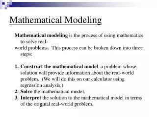
1.3 Mathematical Modeling. A real world problem described using mathematics Recognize real-world problem Collect data Plot data Construct model Explain and predict. Linear Regression. The process of finding a function that best fits the data points is called curve fitting .

E N D
1.3 Mathematical Modeling • A real world problem described using mathematics • Recognize real-world problem • Collect data • Plot data • Construct model • Explain and predict
Linear Regression • The process of finding a function that best fits the data points is called curve fitting. • Curve fitting using linear functions is called linear regression.
Linear Regression on the TI-83 • The first step is to enter the data into the calculator. • Hit STAT and highlight 1:EDIT on the menu list. • Press ENTER
Entering data into the lists • If data is in list, move cursor to highlight list name, press CLEAR followed by ENTER • Enter the x values in L1 and the y values in L2.
Engage the Stat Plot • Press 2nd followed by Y=. • Press ENTER. • Move cursor to highlight On and press ENTER. • Move cursor to highlight scatterplot, and press ENTER. • Make sure the Xlist is L1 and the Ylist is L2.
Adjusting the Window • Standard viewing rectangle is [10,10] xscl=1 and [10,10] yscl=1 • Press WINDOW and enter new dimensions • New window [0,30] xscl=3 and [0,20] yscl=2
Graph data • To view data points, press GRAPH • Data points can be “fitted” by a straight line • Each x tick mark represents 3 years • Each y tick mark represents 2 million households
Find “Best Fit” Linear Function • Press STAT and highlight CALC • Highlight 4:LinReg • Press ENTER
Find Slope and Y Int of Line • Press ENTER a second time • Recall y=mx+bwhere m=slope and b=yint • Note a=slope
Entering “Best Fit” line in Grapher • Press STAT, arrow over to CALC, and highlight 4:LinReg • Press VARS, arrow over to Y-VARS and highlight 1:Function • Press ENTER
Input into Y= Automatically • Highlight 1:Y1 and press ENTER • Press ENTER again
Graph Best Fit Line • Press GRAPH
Use Model to Predict • Use table feature to find prediction • Press 2nd then WINDOW (TBLSET) • Arrow down to change Independent to ASK
Use Table to Find Prediction • Press 2ndGRAPH (TABLE) • Enter 33 since 2003 is 33 years after 1970 • Press ENTER • Interpret answer • Approx. 16.644 million apt households in 2003.