Download
1 / 13
130 likes | 224 Views
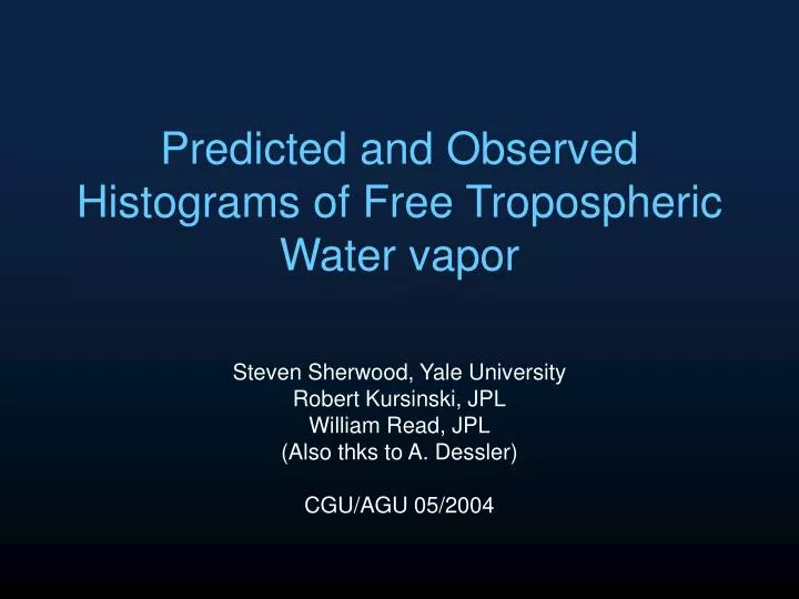
Predicted and Observed Histograms of Free Tropospheric Water vapor. Steven Sherwood, Yale University Robert Kursinski, JPL William Read, JPL (Also thks to A. Dessler) CGU/AGU 05/2004. Water vapor feedback. GCM’s show RH distributions not changing much as climate warms --> positive WVF

E N D
Predicted and Observed Histograms of Free Tropospheric Water vapor Steven Sherwood, Yale University Robert Kursinski, JPL William Read, JPL (Also thks to A. Dessler) CGU/AGU 05/2004
Water vapor feedback • GCM’s show RH distributions not changing much as climate warms --> positive WVF • Can we trust them? Why do they do this?
The “cold trap” model of Relative Humidity • Water vapor near saturation in small moist convective regions; • Water vapor mixing ratio conserved as air leaves; • Dynamics maintains constant (small) difference between temperatures in convective and elsewhere; • Horizontal extent and organization of convective regions, RH within, and transport therefrom are known (…??)
Simulation of vapor from known dynamics Pierrehumbert and Roca, 1998. (See also Sherwood 1996; Salathe and Hartmann 1997)
Stochastic implementation From Clausius Clapeyron eq: Integrated through time: dry is a few days. This gives RH as a function of parcel “age” t. Parcels age until swept into another convective system, where t is reset to zero. If we additionally suppose remoistening is a Poisson process, then Which finally gives
Observed distributions • Upper troposphere: MLS (UARS) v4.9 retrievals from 450-150 hPa (FY 1993) • 3 km resolution, microwave limb emission • Partial cloud penetration • Lower+middle troposphere: GPS (CHAMP) occulations (O ‘91, JAJ ‘92) • 200 m resolution, radio refraction • Full cloud penetration • Diffraction-corrected (C. Ao, R. Mastaler) • These data are preliminary!!
Predicted vs. observed distribution (MLS, 30S-30N) of RH Cloud contamination RH0
Predicted vs. observed distribution (GPS, 30S-30N) of RH RH0
Eulerian implementation (II) • Prefer theory that predicts RH0, ratio, and vs. height, and that accounts for convective ceiling. • Energy + mass conservation constrain dry • A simple, 2-parameter model gets 3/4!: • Simple overturning circulation in energy balance • Precipitation efficiency and/or mixing constant in convective region • Horizontal mixing constant • Still have to prescribe but results not sensitive to it.
EULERIAN MODEL GPS MLS
Model sensitivity RH mean Microphysical parameter RH range Horizontal mixing rate
Conclusions • A comprehensible model of relative humidity does exist • It explains observations of very dry air, convergent histograms, bimodality, and RH min at 400 hPa indicated by MLS and GPS data • It predicts that RH distributions are not very sensitive to cloud microphysical effects, but are somewhat sensitive to how frequently air parcels encounter convection • Further tests of the theory are needed