Download
1 / 5
50 likes | 119 Views
The importance of prefiltering. The estimates are generally biased E{ f T ( )} = W T ( - ) f( ) d Seismic noise horizontal components recorded at UCB Estimated coherence can be 1,0 when no relation

E N D
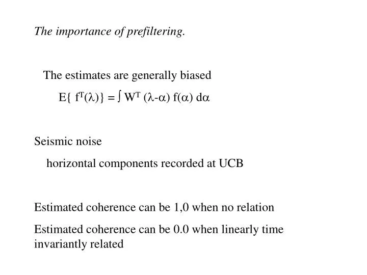
The importance of prefiltering. The estimates are generally biased E{ fT()} = WT (-) f() d Seismic noise horizontal components recorded at UCB Estimated coherence can be 1,0 when no relation Estimated coherence can be 0.0 when linearly time invariantly related
postscript(file="seismic.eps") junkx<-scan("ts_drb.16.dat") junky<-scan("ts_drb.17.dat") par(mfrow=c(2,1)) xaxis<-c(1:2500)*.08 plot(xaxis,junkx,type="l",main="Vertical component seismic noise at Berkeley",xlab="time (sec)",ylab="",las=1) plot(xaxis,junky,type="l",main="West component",xlab="time(sec)",ylab="",las=1) par(mfrow=c(2,3)) junk<-spec.pgram(cbind(junkx,junky),spans=15,taper=0,detrend=F,demean=T,plot=F) junk$freq<-junk$freq/.08 plot(junk$freq,junk$spec[,1],type="l",las=1,main="Vertical noise",xlab="frequency (hertz)",log="y") plot(junk$freq,junk$spec[,2],type="l",las=1,main="West noise",log="y") plot(junk$freq,junk$coh,type="l",ylim=c(0,1),main="Raw data",las=1) abline(h=1-(1-.95)^(1/(.5*(junk$df-2))))
junkxx<-ar(junkx,order.max=2) junkyy<-ar(junky,order.max=2) Junkx<-junkxx$resid Junky<-junkyy$resid Junkx<-Junkx[3:length(Junkx)];Junky<-Junky[3:length(Junky)] Junk<-spec.pgram(cbind(Junkx,Junky),spans=15,taper=0,detrend=F,demean=T,plot=F) Junk$freq<-Junk$freq/.08 plot(Junk$freq,Junk$spec[,1],type="l",las=1,log="y") plot(Junk$freq,Junk$spec[,2],type="l",las=1,log="y") plot(Junk$freq,Junk$coh,type="l",ylim=c(0,1),main="AR(2) residuals",las=1) abline(h=1-(1-.95)^(1/(.5*(junk$df-2)))) graphics.off()