Download
1 / 32
320 likes | 483 Views
Non-exponential Decay of Wavefunctions and Scattering Resonances. Athanasios Petridis Drake University. COLLABORATORS: L. Staunton (Drake Univ.) M. Luban (Iowa State Univ.) J. Vermedahl (Drake Univ.) ACKNOWLEDGEMENTS: K. Bartschat (Drake Univ.) . Outline.

E N D
Non-exponential Decayof Wavefunctions and Scattering Resonances Athanasios Petridis Drake University COLLABORATORS: L. Staunton (Drake Univ.) M. Luban (Iowa State Univ.) J. Vermedahl (Drake Univ.) ACKNOWLEDGEMENTS: K. Bartschat (Drake Univ.)
Outline • Exponential decay • Numerical method • Case studies • Interpretation • Scattering resonances • Conclusions and outlook
V x x L L Exponential decay • A wavefunction initially inside a finite potential well will disperse through the walls if it is not an eigenfunction for this potential: it will decay. • Examples: escape of a particle from a well or decay of a composite object bound by V. V 0 0 Cut HO Cut LC
The probability for finding the particle inside the potential well is • This can also be expressed as
At times much greater than the longest normal-mode oscillation period in the potential it is often assumed that where is the decay width of the system and E=E(p). • With proper normalization where is the decay constant and P0 is the interior probability at t=0.
Numerical Method • We solve the time-dependent Shrödinger equation using the staggered leap-frog method. • We define a grid of n0 points with spacing x, and update the wavefunction at time intervals t. • We evaluate the function at using the stored values at t for every grid point n: t+2t Time 2 1 0
This method is VERY stable numerically but requires small time steps. • Normalization accuracy of 10-9 is achieved (10-12 per grid point). • Reflecting boundary conditions are used. This requires very large grid to avoid interference of the waves reflected on the wall with the wave inside the potential well. • The initial wavefunction can be “still” or have a group velocity (v0).
Testing the numerical method: • Verified that the square of the width of a minimum packet increases quadratically with time. • Verified that in a harmonic oscillator potential the magnitude squared of any linear combination of eigenfunctions with no initial group velocity will retrieve itself after exactly one classical period.
T/4 T/2
Case Studies • Cut harmonic oscillator potential (Cut HO). • Cut linear confining potential (Cut LC). • Initial wave functions: (1) general gaussian (2) HO ground state. • Initial group velocities: (1) zero (2) 1 unit. • Snapshots of |(x,t)|2 , Pin(t), dPin(t)/dt
General features of the results: • The wavefunction “breaths” inside the potential “exhaling” wavepackets that travel away in both directions. This is due to reflection and transmission of wave-components off the through the walls. • The probability, Pin, exhibits “plateaux” which appear to be periodic. They correspond to the “inhaling” mode of the function. • Following the “plateaux”-like behavior, the derivative of Pin fluctuates as well. • There is a transition time for the fluctuations to settle into a steady frequency.
Can this behavior be attributed to the sharpness of the potential (infinite classical force at the sharp edges)? • J. Vermedahl has rounded the corners of the cut HO potential and added a smooth drop to zero: the results are qualitatively the same! • However: the slope of the curve and the period and size of the fluctuations depend on the shape and magnitude of the potential and the Initial Conditions ((x,0), v0).
LC (cut at 25) (x,0)=gaussian (width=60, v0=0) • Important observation: at large times the probability DOES decay exponentially.
Interpretation • Generally, there is no complete analytical calculation. We are in the process of cut HO analytical calculations. • The probability function versus time appears to consist of a “median” curve with oscillations of fixed period around it. • The median deviates from a simple exponential at “short” times. • The amplitude of the oscillations appears to decrease with time. • There may be some initial “transition” interval.
LC (cut at 100), (x,0)=gaussian (width=60, v0=0) K = 0.1089 N1 = 1.0015 N2 = 0.9892 W = 0.1911 C = 0.0084 L = 0.0046 Q = 0.7882 S(t) starts slightly negative and becomes positive with time.
There are FIVE time scales: 1. The overall (long time) decay constant. 2. The time it takes for the median curve to become a simple exponential. 3. The dominant period of oscillations. 4. The time it takes for the oscillations to damp out. 5. The initial oscillation transient time.
Scattering Resonances • One application: Nuclear decay. • Resonant scattering (production-decay of baryons in pion-proton scattering). • In the CM frame E=m(ħ=c=1). For large t (Breit-Wigner curve)
LC (cut at 100), (x,0)=gaussian (width=60, v0=0) standard modified
Conclusions and outlook • There are deviations from exponential decay at small times.They can be connected with auto-correlations and “breathing” of the wavefunction. • They may be visible in time and energy domains. • Analytical understanding is needed. An analysis of the wavefunction on eigenfunctions would show oscillatory behavior. • The relativistic Dirac equation can be studied.