Download
1 / 32
320 likes | 326 Views
Learn about the quick-sort algorithm, its execution example, and its worst-case running time. Also, explore the lower bound on runtimes for comparison-based sorting algorithms.

E N D
7 4 9 6 2 2 4 6 7 9 4 2 2 4 7 9 7 9 2 2 9 9 Chapter 4: Sorting Sorting Fun
What We’ll Do • Quick Sort • Lower bound on runtimes for comparison based sort • Radix and Bucket sort Sorting Fun
7 4 9 6 2 2 4 6 7 9 4 2 2 4 7 9 7 9 2 2 9 9 Quick-Sort Sorting Fun
Quick-sort is a randomized sorting algorithm based on the divide-and-conquer paradigm: Divide: pick a random element x (called pivot) and partition S into L elements less than x E elements equal x G elements greater than x Recur: sort L and G Conquer: join L, Eand G Quick-Sort x x L G E x Sorting Fun
Partition Algorithmpartition(S,p) Inputsequence S, position p of pivot Outputsubsequences L,E, G of the elements of S less than, equal to, or greater than the pivot, resp. L,E, G empty sequences x S.remove(p) whileS.isEmpty() y S.remove(S.first()) ify<x L.insertLast(y) else if y=x E.insertLast(y) else{ y > x } G.insertLast(y) return L,E, G • We partition an input sequence as follows: • We remove, in turn, each element y from S and • We insert y into L, Eor G,depending on the result of the comparison with the pivot x • Each insertion and removal is at the beginning or at the end of a sequence, and hence takes O(1) time • Thus, the partition step of quick-sort takes O(n) time Sorting Fun
Quick-Sort Tree • An execution of quick-sort is depicted by a binary tree • Each node represents a recursive call of quick-sort and stores • Unsorted sequence before the execution and its pivot • Sorted sequence at the end of the execution • The root is the initial call • The leaves are calls on subsequences of size 0 or 1 7 4 9 6 2 2 4 6 7 9 4 2 2 4 7 9 7 9 2 2 9 9 Sorting Fun
Execution Example • Pivot selection 7 2 9 4 3 7 6 11 2 3 4 6 7 8 9 7 2 9 4 2 4 7 9 3 8 6 1 1 3 8 6 9 4 4 9 3 3 8 8 2 2 9 9 4 4 Sorting Fun
Execution Example (cont.) • Partition, recursive call, pivot selection 7 2 9 4 3 7 6 11 2 3 4 6 7 8 9 2 4 3 1 2 4 7 9 3 8 6 1 1 3 8 6 9 4 4 9 3 3 8 8 2 2 9 9 4 4 Sorting Fun
Execution Example (cont.) • Partition, recursive call, base case 7 2 9 4 3 7 6 11 2 3 4 6 7 8 9 2 4 3 1 2 4 7 3 8 6 1 1 3 8 6 11 9 4 4 9 3 3 8 8 9 9 4 4 Sorting Fun
Execution Example (cont.) • Recursive call, …, base case, join 7 2 9 4 3 7 6 11 2 3 4 6 7 8 9 2 4 3 1 1 2 3 4 3 8 6 1 1 3 8 6 11 4 334 3 3 8 8 9 9 44 Sorting Fun
Execution Example (cont.) • Recursive call, pivot selection 7 2 9 4 3 7 6 11 2 3 4 6 7 8 9 2 4 3 1 1 2 3 4 7 9 7 1 1 3 8 6 11 4 334 8 8 9 9 9 9 44 Sorting Fun
Execution Example (cont.) • Partition, …, recursive call, base case 7 2 9 4 3 7 6 11 2 3 4 6 7 8 9 2 4 3 1 1 2 3 4 7 9 7 1 1 3 8 6 11 4 334 8 8 99 9 9 44 Sorting Fun
Execution Example (cont.) • Join, join 7 2 9 4 3 7 6 1 1 2 3 4 67 7 9 2 4 3 1 1 2 3 4 7 9 7 1779 11 4 334 8 8 99 9 9 44 Sorting Fun
Worst-case Running Time • The worst case for quick-sort occurs when the pivot is the unique minimum or maximum element • One of L and G has size n - 1 and the other has size 0 • The running time is proportional to the sum n+ (n- 1) + … + 2 + 1 • Thus, the worst-case running time of quick-sort is O(n2) number of comparisons in partition step … Sorting Fun
Consider a recursive call of quick-sort on a sequence of size s Good call: the sizes of L and G are each less than 3s/4 Bad call: one of L and G has size greater than 3s/4 A call is good with probability 1/2 1/2 of the possible pivots cause good calls: 1 2 3 4 5 6 7 8 9 10 11 12 13 14 15 16 Expected Running Time 7 2 9 4 3 7 6 1 9 7 2 9 4 3 7 6 1 1 7 2 9 4 3 7 6 2 4 3 1 7 9 7 1 1 Good call Bad call Bad pivots Good pivots Bad pivots Sorting Fun
Probabilistic Fact: The expected number of coin tosses required in order to get k heads is 2k For a node of depth i, we expect i/2 ancestors are good calls The size of the input sequence for the current call is at most (3/4)i/2n Since each good call shrinks size to at most 3/4 of previous size Expected Running Time, Part 2 • Therefore, we have • For a node of depth 2log4/3n, the expected input size is one • The expected height of the quick-sort tree is O(log n) • The amount or work done at the nodes of the same depth is O(n) • Thus, the expected running time of quick-sort is O(n log n) Sorting Fun
Sorting Lower Bound Sorting Fun
Many sorting algorithms are comparison based. They sort by making comparisons between pairs of objects Examples: bubble-sort, selection-sort, insertion-sort, heap-sort, merge-sort, quick-sort, ... Let us therefore derive a lower bound on the running time of any algorithm that uses comparisons to sort a set S of n elements, x1, x2, …, xn. Is xi < xj? no yes Comparison-Based Sorting (§ 4.4) Assume that the xi are distinct, which is not a restriction Sorting Fun
Let us just count comparisons then. First, we can map any comparison based sorting algorithm to a decision tree as follows: Let the root node of the tree correspond to the first comparison, (is xi < xj?), that occurs in the algorithm. The outcome of the comparison is either yes or no. If yes we proceed to another comparison, say xa< xb? We let this comparison correspond to the left child of the root. If no we proceed to the comparison xc < xd? We let this comparison correspond to the right child of the root. Each of those comparisons can be either yes or no… Counting Comparisons Sorting Fun
Each possible permutation of the set S will cause the sorting algorithm to execute a sequence of comparisons, effectively traversing a path in the tree from the root to some external node The Decision Tree Sorting Fun
Paths Represent Permutations • Fact: Each external node v in the tree can represent the sequence of comparisons for exactly one permutation of S • If P1 and P2 are different permutations, then there is at least one pair xi, xj with xi before xj in P1 and xi after xj in P2 • For both P1 and P2 to end up at v, this means every decision made along the way resulted in the exact same outcome. • We have a decision tree, so no cycles! • This cannot occur if the sorting algorithm behaves correctly, because in one permutation xi started before xj and in the other their order was reversed (remember, they cannot be equal) Sorting Fun
Decision Tree Height • The height of this decision tree is a lower bound on the running time • Every possible input permutation must lead to a separate leaf output (by previous slide). • There are n! permutations, so there are n! leaves. • Since there are n!=1*2*…*n leaves, the height is at least log (n!) Sorting Fun
The Lower Bound • Any comparison-based sorting algorithms takes at least log (n!) time • Therefore, any such algorithm takes time at least • Since there are at least n/2 terms larger than n/2 in n! • That is, any comparison-based sorting algorithm must run no faster than O(n log n) time in the worst case. Sorting Fun
Bucket-Sort and Radix-Sort 1, c 3, a 3, b 7, d 7, g 7, e 0 1 2 3 4 5 6 7 8 9 B Sorting Fun
Let be S be a sequence of n (key, element) items with keys in the range [0, N- 1] Bucket-sort uses the keys as indices into an auxiliary array B of sequences (buckets) Phase 1: Empty sequence S by moving each item (k, o) into its bucket B[k] Phase 2: For i = 0, …,N -1, move the items of bucket B[i] to the end of sequence S Analysis: Phase 1 takes O(n) time Phase 2 takes O(n+ N) time Bucket-sort takes O(n+ N) time Bucket-Sort (§ 4.5.1) AlgorithmbucketSort(S,N) Inputsequence S of (key, element) items with keys in the range [0, N- 1]Outputsequence S sorted by increasing keys B array of N empty sequences whileS.isEmpty() f S.first() (k, o) S.remove(f) B[k].insertLast((k, o)) for i 0 toN -1 whileB[i].isEmpty() f B[i].first() (k, o) B[i].remove(f) S.insertLast((k, o)) Sorting Fun
7, d 1, c 3, a 7, g 3, b 7, e 1, c 3, a 3, b 7, d 7, g 7, e B 0 1 2 3 4 5 6 7 8 9 1, c 3, a 3, b 7, d 7, g 7, e Example • Key range [0, 9] Phase 1 Phase 2 Sorting Fun
Key-type Property The keys are used as indices into an array and cannot be arbitrary objects No external comparator Stable Sort Property The relative order of any two items with the same key is preserved after the execution of the algorithm Extensions Integer keys in the range [a, b] Put item (k, o) into bucketB[k - a] String keys from a set D of possible strings, where D has constant size (e.g., names of the 50 U.S. states) Sort D and compute the rank r(k)of each string k of D in the sorted sequence Put item (k, o) into bucket B[r(k)] Properties and Extensions Sorting Fun
Lexicographic Order • A d-tuple is a sequence of d keys (k1, k2, …, kd), where key ki is said to be the i-th dimension of the tuple • Example: • The Cartesian coordinates of a point in space are a 3-tuple • The lexicographic order of two d-tuples is recursively defined as follows (x1, x2, …, xd) < (y1, y2, …, yd)x1 <y1 x1=y1 (x2, …, xd) < (y2, …, yd) I.e., the tuples are compared by the first dimension, then by the second dimension, etc. Sorting Fun
Lexicographic-Sort AlgorithmlexicographicSort(S) Inputsequence S of d-tuplesOutputsequence S sorted in lexicographic order for i ddownto 1 stableSort(S, Ci) • Let Ci be the comparator that compares two tuples by their i-th dimension • Let stableSort(S, C) be a stable sorting algorithm that uses comparator C • Lexicographic-sort sorts a sequence of d-tuples in lexicographic order by executing d times algorithm stableSort, one per dimension • Lexicographic-sort runs in O(dT(n)) time, where T(n) is the running time of stableSort Example: (7,4,6) (5,1,5) (2,4,6) (2, 1, 4) (3, 2, 4) (2, 1, 4) (3, 2, 4) (5,1,5) (7,4,6) (2,4,6) (2, 1, 4) (5,1,5) (3, 2, 4) (7,4,6) (2,4,6) (2, 1, 4) (2,4,6) (3, 2, 4) (5,1,5) (7,4,6) Sorting Fun
Radix-sort is a specialization of lexicographic-sort that uses bucket-sort as the stable sorting algorithm in each dimension Radix-sort is applicable to tuples where the keys in each dimension i are integers in the range [0, N- 1] Radix-sort runs in time O(d( n+ N)) Radix-Sort (§ 4.5.2) AlgorithmradixSort(S, N) Inputsequence S of d-tuples such that (0, …, 0) (x1, …, xd) and (x1, …, xd) (N- 1, …, N- 1) for each tuple (x1, …, xd) in SOutputsequence S sorted in lexicographic order for i ddownto 1 bucketSort(S, N) Sorting Fun
Radix-Sort for Binary Numbers • Consider a sequence of nb-bit integers x=xb- 1 … x1x0 • We represent each element as a b-tuple of integers in the range [0, 1] and apply radix-sort with N= 2 • This application of the radix-sort algorithm runs in O(bn) time • For example, we can sort a sequence of 32-bit integers in linear time AlgorithmbinaryRadixSort(S) Inputsequence S of b-bit integers Outputsequence S sorted replace each element x of S with the item (0, x) for i 0 tob - 1 replace the key k of each item (k, x) of S with bit xi of x bucketSort(S, 2) Sorting Fun
1001 1001 1001 0001 0010 0010 0010 1101 0001 1110 1101 1001 0001 0010 1001 1101 0001 0010 1101 1101 1110 1110 1110 1110 0001 Example • Sorting a sequence of 4-bit integers Sorting Fun