Download

1 / 32
320 likes | 493 Views
Migration. “Gene flow” movement of individuals between populations may be one-way; donor population and recipient population may be two-way may involve more than two populations. Migration. Simplest case: one-way migration. Population 1 Population 2 p = 0.9 p = 0.3

E N D
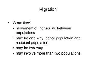
Migration • “Gene flow” • movement of individuals between populations • may be one-way; donor population and recipient population • may be two-way • may involve more than two populations
Migration Simplest case: one-way migration Population 1 Population 2 p = 0.9 p = 0.3 q = 0.1 q = 0.7 genotype frequencies: AA AB BB AA AB BB .81 .18 .01 .09 .42 .49 If migration is from population 1 to 2, 81% of the migrants will be AA’s. This will cause p in population 2 to increase.
Migration; one-way: Population 1 Population 2 p = 0.9 p = 0.3 q = 0.1 q = 0.7 Dqr = m(qm - qr) qr new = qr + Dq if m = 15%: Dq = 0.15(0.1 - 0.7) = -0.09 qr = 0.7 + (-0.09) = 0.61
Migration; two-way Population 1 Population 2 p = 0.9 p = 0.3 q = 0.1 q = 0.7 If there is migration from 1 into 2 as well as from 2 into 1, the populations will eventually become one population. They will reach an equilibrium: q = (q1 + q2) / 2 i.e. q at equilibrium will be the average of all the q’s ^
Random Genetic Drift • Due to small population size • deviations in allele frequencies simply due to chance • sometimes called “Sampling error” • Compare to a small family: 4 children • 1/2 should be boys, 1/2 girls • not unusual for all to be girls or 3 boys and 1 girl, etc.
Random Genetic Drift • VERY simplistic example: population of 4 individuals: AA AB AB BB p = q = 0.5 Suppose AA mates with BB; AB with AB possible offspring: AA x BB --> AB AB x AB --> AA, AB, & BB
Random Genetic Drift If each pair produces two offspring, we might see something like this in the next generation: AB AB AA AB p1 = 5/8 = 0.625 The next generation might just as easily have been: AB AB AB BB p1 = 3/8 = 0.375
Random Genetic Drift • The smaller the population, the more noticeable the effects of drift • Changes are totally random • If a population is small enough, the effects of drift may swamp the other four forces, even selection
Non-Random Mating • Not all matings are equally likely to occur • Assortative mating • Negative assortative mating • individuals tend to mate with others of different genotype • AA x AB; AA x BB; AB x BB; AA x BB • not terribly common
Non-Random Mating • positive assortative mating • individuals tend to mate only with others of like genotype • AA x AA; AB x AB; BB x BB • Inbreeding is a type of p.a.m. • self-fertilization is the most extreme case
Inbreeding AA x AA AB x AB BB x BB AA 1/4AA 1/2 AB 1/4 BB BB Net increase in homozygotes; decrease in heterozygotes Effect on genotype frequencies? Why are consanguineous matings not a good idea?
Mutation • Ultimate source of all new genetic variation • All new alleles arise through mutation • Changes in allele frequencies due to mutation alone are extremely slow
Mutation Original population: all homozygous for allele A No genetic variability; no polymorphism p = 1.0; q = 0 A mutation occurs changing allele A in to allele B. This occurs at a rate we will call m. q will now be equal to that fraction of p that mutated: Dq = mp
Mutation q1 = q0 + Dq Dq = mp Example: p0 = 1.0 m = 10-5 q1 = 0.0 + 0.00001 = 0.00001 p1 = 0.99999 Dq = (10-5) (1.0) = 0.00001
Mutation That’s not even taking into account back mutation! If A can mutate to B; B can back mutate to A! This slows down the accumulation of B alleles even more: m A B n Dq = mp - nq
p0 = 0.9 q0 = 0.1 m = 10-5 n = 10-6 Dq = mp - nq Dq = (10-5)(0.9) - (10-6)(0.1) = 0.0000089 p1 = 0.8999911
Selection • Differential reproduction • those individuals best able to survive and reproduce will do so more often than others • if the differences in ability are genetic, the genes conferring the higher ability will increase in frequency
Fitness • Selection is based on differences in fitness • Fitness refers to the ability to survive and produce offspring • Fitness is a measure of viable offspring produced
Fitness • Darwinian fitness is the average number of offspring left by a genotype • AA AB BB • 10 8 4
Fitness • Relative fitness (w) calculates fitness in relation to the most fit genotype • most fit genotype has a fitness of 1 AA AB BB 10 8 4 Darwinian 10/10 8/10 4/10 1.0 0.8 0.4 Relative
Fitness vs. Selection Coefficient • A second way to look a fitness is the selection coefficient • the amount of selection against a genotype • s = 1 - w AA AB BB w: 1 0.8 0.4 s: 0 0.2 0.6
AA AB BB freq.: p2 2pq q2 w: 1 0.8 0.4 With a difference in fitness, each genotype no longer has an equal likelihood of contributing to the gene pool of the next generation. The contribution to the next generation is a result of frequency times fitness.
Mean Population Fitness w = mean population fitness = how fit the population is as a whole w = p2 (wAA) + 2pq (wAB) + q2 (wBB) As selection proceeds, w should increase.
Allele frequencies at the next generation: pn2 (wAA) + pq (wAB) pn+1 = -------------------------------- w
Example: AA AB BB s: 0 0.1 0.5 w: 1 0.9 0.5 p0 = q0 = 0.5 (.5)2 (1) + (.5)(.5)(.9) p1 = ------------------------------------------------ (.5)2 (1) + 2(.5)(.5)(.9) + (.5)2 (.5) p1 = .475/.825 = 0.58 q1 = 0.42
Fisher’s Fundamental Theorem The rate of change of allele frequencies is directly proportional to the amount of genetic variability. p = q ; highest amount of variability for two alleles greatest amount of change in p or q from one generation to the next
Example: AA AB BB w: 1 0.9 0.5 p0 = 0.5 p1 = 0.58 8% change pn = 0.9 pn + 1 = ?
Selection against a recessive lethal AA Aa aa s: 0 0 1 w: 1 1 0 p = 0.90; q = 0.10
Selection against a dominant lethal AA Aa aa s: 1 1 0 w: 0 0 1 p = 0.90; q = 0.10
Heterosis or heterozygote advantage • Way for selection to maintain a stable equilibrium with polymorphism • BOTH alleles selected for • Heterozygote more fit than either homozygote • Keeps “harmful” allele at a fairly high frequency
Sickle cell anemia • In areas where malaria is endemic, Ss have a fitness advantage • Plasmodium causing malaria cannot survive as well w/ sickled cells in bloodstream • SS: no anemia; susceptible to malaria • ss: anemia; no malaria • Ss: no anemia; resistant to malaria
SS Ss ss w: .7 1 .1 s: .3 0 .9 s2 p = ----------- s1 + s2 ^ .9 p = ---------- = .75 .3 + .9 ^