Download
1 / 65
650 likes | 788 Views
Brief Introduction to the Theory of Evolution. Anders Gorm Pedersen Molecular Evolution Group Center for Biological Sequence Analysis gorm@cbs.dtu.dk. Classification: Linnaeus. Carl Linnaeus 1707-1778. Classification: Linnaeus. Hierarchical system Kingdom Phylum Class Order

E N D
Brief Introduction to the Theory of Evolution Anders Gorm Pedersen Molecular Evolution Group Center for Biological Sequence Analysis gorm@cbs.dtu.dk
Classification: Linnaeus Carl Linnaeus 1707-1778
Classification: Linnaeus • Hierarchical system • Kingdom • Phylum • Class • Order • Family • Genus • Species
Classification depicted as a tree Species Genus Family Order Class
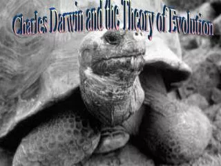
Theory of evolution Charles Darwin 1809-1882
Phylogenetic basis of systematics • Linnaeus: Ordering principle is God. • Darwin: Ordering principle is shared descent from common ancestors. • Today, systematics is explicitly based on phylogeny.
Darwin’s four postulates • More young are produced each generation than can survive to reproduce. • Individuals in a population vary in their characteristics. • Some differences among individuals are based on genetic differences. • Individuals with favorable characteristics have higher rates of survival and reproduction. • Evolution by means of natural selection • Presence of ”design-like” features in organisms: • quite often features are there “for a reason”
Theory of evolution as the basis of biological understanding ”Nothing in biology makes sense, except in the light of evolution. Without that light it becomes a pile of sundry facts - some of them interesting or curious but making no meaningful picture as a whole” T. Dobzhansky
Phylogenetic Reconstruction:Distance Matrix Methods Anders Gorm Pedersen Molecular Evolution Group Center for Biological Sequence Analysis Technical University of Denmark gorm@cbs.dtu.dk
Trees: representations Three different representations of the same tree
Trees: rooted vs. unrooted • A rooted tree has a single node (the root) that represents a point in time that is earlier than any other node in the tree. • A rooted tree has directionality (nodes can be ordered in terms of “earlier” or “later”). • In the rooted tree, distance between two nodes is represented along the time-axis only (the second axis just helps spread out the leafs) Early Late
Trees: rooted vs. unrooted • A rooted tree has a single node (the root) that represents a point in time that is earlier than any other node in the tree. • A rooted tree has directionality (nodes can be ordered in terms of “earlier” or “later”). • In the rooted tree, distance between two nodes is represented along the time-axis only (the second axis just helps spread out the leafs) Early Late
Trees: rooted vs. unrooted • A rooted tree has a single node (the root) that represents a point in time that is earlier than any other node in the tree. • A rooted tree has directionality (nodes can be ordered in terms of “earlier” or “later”). • In the rooted tree, distance between two nodes is represented along the time-axis only (the second axis just helps spread out the leafs) Early Late
Trees: rooted vs. unrooted • In unrooted trees there is no directionality: we do not know if a node is earlier or later than another node • Distance along branches directly represents node distance
Trees: rooted vs. unrooted • In unrooted trees there is no directionality: we do not know if a node is earlier or later than another node • Distance along branches directly represents node distance
A A G C G T T G G G C A A B A G C G T T T G G C A A C A G C T T T G T G C A A D A G C T T T T T G C A A 1 2 3 DNA and protein sequences Homologous characters inferred from alignment. Other molecular data: absence/presence of restriction sites, DNA hybridization data, antibody cross-reactivity, etc. (but losing importance due to cheap, efficient sequencing). Molecular phylogeny
Morphology vs. molecular data African white-backed vulture (old world vulture) Andean condor (new world vulture) New and old world vultures seem to be closely related based on morphology. Molecular data indicates that old world vultures are related to birds of prey (falcons, hawks, etc.) while new world vultures are more closely related to storks Similar features presumably the result of convergent evolution
Molecular data: single-celled organisms Molecular data useful for analyzing single-celled organisms (which have only few prominent morphological features).
Distance Matrix Methods • Construct multiple alignment of sequences • Construct table listing all pairwise differences (distance matrix) • Construct tree from pairwise distances Gorilla : ACGTCGTA Human : ACGTTCCT Chimpanzee: ACGTTTCG Ch 1 1 1 Hu 2 Go
Finding Optimal Branch Lengths S2 S1 a c b e d S3 S4 Distance along tree Observed distance D12 d12 = a + b + c D13 d13 = a + d D14 d14 = a + b + e D23 d23 = d + b + c D24 d24 = c + e D34 d34 = d + b + e Goal:
Exercise (handout) • Construct distance matrix (count different positions) • Reconstruct tree and find best set of branch lengths
Optimal Branch Lengths: Least Squares • Fit between given tree and observed distances can be expressed as “sum of squared differences”: Q = (Dij - dij)2 • Find branch lengths that minimize Q - this is the optimal set of branch lengths for this tree. S2 S1 a c b e d S3 S4 Distance along tree j>i D12 d12 = a + b + c D13 d13 = a + d D14 d14 = a + b + e D23 d23 = d + b + c D24 d24 = c + e D34 d34 = d + b + e Goal:
Optimal Branch Lengths: Least Squares • Longer distances associated with larger errors • Squared deviation may be weighted so longer branches contribute less to Q: Q = (Dij - dij)2 • Power (n) is typically 1 or 2 S2 S1 a c b e d S3 S4 Distance along tree D12 d12 = a + b + c D13 d13 = a + d D14 d14 = a + b + e D23 d23 = d + b + c D24 d24 = c + e D34 d34 = d + b + e Dijn Goal:
Least Squares Optimality Criterion • Search through all (or many) tree topologies • For each investigated tree, find best branch lengths using least squares criterion • Among all investigated trees, the best tree is the one with the smallest sum of squared errors. • Least squares criterion used both for finding branch lengths on individual trees, and for finding best tree.
Minimum Evolution Optimality Criterion • Search through all (or many) tree topologies • For each investigated tree, find best branch lengths using least squares criterion • Among all investigated trees, the best tree is the one with the smallest sum of branch lengths (the shortest tree). • Least squares criterion used for finding branch lengths on individual trees, minimum tree length used for finding best tree.
How many unrooted trees are there? • There is only one way of con-structing the first tree. This tree has 3 tips and 3 branches • Each time an extra taxon is added, two branches are created. • A tree with n tips will therefore have the following number of branches: nbranches = 3+(n-3)*2 = 3+2n-6 = 2n-3 A B C A B D C
How many unrooted trees are there? • A tree with n tips has 2n-3 branches • For each tree with n tips, we can therefore construct 2n-3 derived trees (with n+1 tips). • The number of unrooted trees with n+1 tips is therefore: (2i-3) = 1 x 3 x 5 x 7 x ... n i=2
Heuristic search • Construct initial tree; determine sum of squares • Construct set of “neighboring trees” by making small rearrangements of initial tree; determine sum of squares for each neighbor • If any of the neighboring trees are better than the initial tree, then select it/them and use as starting point for new round of rearrangements. (Possibly several neighbors are equally good) • Repeat steps 2+3 until you have found a tree that is better than all of its neighbors. • This tree is a “local optimum” (not necessarily a global optimum!)
Types of rearrangement I: nearest neighbor interchange (NNI) Original tree Two neighbors per internal branch: tree with n tips has 2(n-3) neighbors (For example, a tree with 20 tips has 34 neighbbors)
Types of rearrangement II: subtree pruning and regrafting (SPR)
Types of rearrangement III: tree bisection and reconnection (TBR)
Clustering Algorithms • Starting point: Distance matrix • Cluster least different pair of sequences: • Tree: pair connected to common ancestral node, compute branch lengths from ancestral node to both descendants • Distance matrix: combine two entries into one. Compute new distance matrix, by finding distance from new node to all other nodes • Repeat until all nodes are linked • Results in only one tree, there is no measure of tree-goodness.
Neighbor Joining Algorithm • For each tip compute ui = jDij/(n-2) (this is essentially the average distance to all other tips, except the denominator is n-2 instead of n) • Find the pair of tips, i and j, where Dij-ui-uj is smallest • Connect the tips i and j, forming a new ancestral node. The branch lengths from the ancestral node to i and j are: vi = 0.5 Dij + 0.5 (ui-uj) vj = 0.5 Dij + 0.5 (uj-ui) • Update the distance matrix: Compute distance between new node and each remaining tip as follows: Dij,k = (Dik+Djk-Dij)/2 • Replace tips i and j by the new node which is now treated as a tip • Repeat until only two nodes remain.
Superimposed Substitutions • Actual number of evolutionary events: 5 • Observed number of differences: 2 • Distance is (almost) always underestimated ACGGTGC C T GCGGTGA
Model-based correction for superimposed substitutions • Goal: try to infer the real number of evolutionary events (the real distance) based on • Observed data (sequence alignment) • A model of how evolution occurs
Jukes and Cantor Model • Four nucleotides assumed to be equally frequent (f=0.25) • All 12 substitution rates assumed to be equal • Under this model the corrected distance is: DJC = -0.75 x ln(1-1.33 x DOBS) • For instance: DOBS=0.43 => DJC=0.64
Neighbor Joining Algorithm • For each tip compute ui = jDij/(n-2) (this is essentially the average distance to all other tips, except the denominator is n-2 instead of n) • Find the pair of tips, i and j, where Dij-ui-uj is smallest • Connect the tips i and j, forming a new ancestral node. The branch lengths from the ancestral node to i and j are: vi = 0.5 Dij + 0.5 (ui-uj) vj = 0.5 Dij + 0.5 (uj-ui) • Update the distance matrix: Compute distance between new node and each remaining tip as follows: Dij,k = (Dik+Djk-Dij)/2 • Replace tips i and j by the new node which is now treated as a tip • Repeat until only two nodes remain.
Neighbor Joining Algorithm Dij-ui-uj
Neighbor Joining Algorithm Dij-ui-uj