Download
1 / 231
2.42k likes | 3.08k Views
Individual. Bulk (Grain Size Distribution). }. Secondary properties that are related to the others. Chapter 2. Grain Texture. Clastic sediment and sedimentary rocks are made up of discrete particles.

E N D
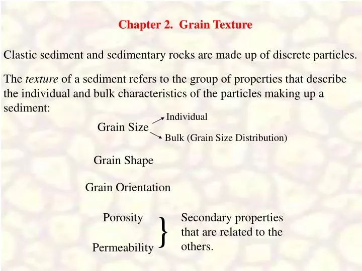
Individual Bulk (Grain Size Distribution) } Secondary properties that are related to the others. Chapter 2. Grain Texture Clastic sediment and sedimentary rocks are made up of discrete particles. The texture of a sediment refers to the group of properties that describe the individual and bulk characteristics of the particles making up a sediment: Grain Size Grain Shape Grain Orientation Porosity Permeability
These properties collectively make up the texture of a sediment or sedimentary rock. Each can be used to infer something of: The history of a sediment. The processes that acted during transport and deposition of a sediment. The behavior of a sediment. This section focuses on each of these properties, including: Methods of determining the properties. The terminology used to describe the properties. The significance of the properties.
Grain Size I. Grain Volume (V) a) Based on the weight of the particle: Where: m is the mass of the particle. V is the volume of the particle. rs is the density of the material making up the particle. (r is the lower case Greek letter rho). 1. Weigh the particle to determine m. 2. Determine or assume a density. (density of quartz = 2650kg/m3) 3. Solve for V. Error due to error in assumed density; Porous material will have a smaller density and less solid volume so this method will underestimate the overall volume.
Accuracy depends on how accurately the displaced volume can be measured. Not practical for very small grains. For porous materials this method will underestimate the external volume of the particle.
c) Based on dimensions of the particle. Where: d is the diameter of the particle And the particle is a perfect sphere. Measure the diameter of the particle and solve for V. Problem: natural particles are rarely spheres.
II. Linear dimensions. a) Direct Measurement Natural particles normally have irregular shapes so that it is difficult to determine what linear dimensions should be measured. Most particles are not spheres so we normally assume that they can be described as triaxial ellipsoids that are described in terms of three principle axes: dL or a-axis longest dimension. dI or b-axis intermediate dimension. dS or c-axis shortest dimension.
The maximum projection area is the area of intersection of the plane with the particle. To define the three dimensions requires a systematic method so that results by different workers will be consistent. Sedimentologists normally use the Maximum Tangent Rectangle Method. Step 1. Determine the plane of maximum projection for the particle. -an imaginary plane passing through the particle which is in contact with the largest surface area of the particle.
maximum tangent rectangle Step 2. Determine the maximum tangent rectangle for the maximum projection area. -a rectangle with sides having maximum tangential contact with the perimeter of the maximum projection area (the outline of the particle)
Step 2. Determine the maximum tangent rectangle for the maximum projection area. -a rectangle with sides having maximum tangential contact with the perimeter of the maximum projection area (the outline of the particle) dL is the length of the rectangle. dI is the width of the rectangle.
Step 3. Rotate the particle so that you view the surface that is at right angles to the plane of maximum projection. dS is the longest distance through the particle in the direction normal to the plane of maximum projection.
The volume of a triaxial ellipsoid is given by: p dL x dI x dS V = 6
Click here to see how a thin section is made. http://faculty.gg.uwyo.edu/heller/Sed%20Strat%20Class/SedStratL1/thin_section_mov.htm For fine particles only dL and dI can be measured in thin sections. Thin sections are 30 micron (30/1000 mm) thick slices of rock through which light can be transmitted.
Axes lengths measured in thin section are “apparent dimensions” of the particle. The length measured in thin section depends on where in the particle that the plane of the thin section passes.
Axes lengths measured in thin section are “apparent dimensions” of the particle. The length measured in thin section depends on where in the particle that the plane of the thin section passes.
Axes lengths measured in thin section are “apparent dimensions” of the particle. The length measured in thin section depends on where in the particle that the plane of the thin section passes. For a spherical particle its true diameter is only seen in thin section when the plane of the thin section passes through the centre of the particle.
V1 = volume of the sphere. V2 = volume of a particle. (a triaxial ellipsoid) Therefore: The three axes lengths that are commonly measured are often expressed as a single dimension known as the nominal diameter of a particle (dn): dn is the diameter of the sphere with volume (V1) equal the volume (V2) of the particle with axes lengths dL, dI and dS. By the definition of nominal diameter, V1 = V2
Therefore: Nominal diameter dn can be solved by rearranging the terms:
b) Sieving A sample is passed through a vertically stacked set of square-holed screens (sieves). Used to determine the grain size distribution (a bulk property of a sediment).
A set of screens are stacked, largest holes on top, smallest on the bottom and shaken in a sieve shaker (Rotap shakers are recommended). Grains that are larger than the holes remain on a screen and the smaller grains pass through, collecting on the screen with holes just smaller than the grains. The grains collected on each screen are weighed to determine the weight of sediment in a given range of size. The later section on grain size distributions will explain the method more clearly. Details of the sieving method are given in Appendix I of the course notes.
III. Settling Velocity Another expression of the grain size of a sediment is the settling velocity of the particles. Settling velocity (w; the lower case Greek letter omega ): the terminal velocity at which a particles falls through a vertical column of still water. Possibly a particularly meaningful expression of grain size as many sediments are deposited from water. When a particle is dropped into a column of fluid it immediately accelerates to some velocity and continues falling through the fluid at that velocity (often termed the terminal settling velocity).
The speed of the terminal settling velocity of a particle depends on properties of both the fluid and the particle: Properties of the particle include: The size if the particle (d). The density of the material making up the particle (rs). The shape of the particle.
a) Direct measurement Settling velocity can be measured using settling tubes: a transparent tube filled with still water. In a very simple settling tube: A particle is allowed to fall from the top of a column of fluid, starting at time t1. The particle accelerates to its terminal velocity and falls over a vertical distance, L, arriving there at a later time, t2. The settling velocity can be determined:
A variety of settling tubes have been devised with different means of determining the rate at which particles fall. Some apply to individual particles while others use bulk samples. i) Tube length: the tube must be long enough so that the length over which the particle initially accelerates is small compared to the total length over which the terminal velocity is measured. Important considerations for settling tube design include: Otherwise, settling velocity will be underestimated.
ii) Tube diameter: the diameter of the tube must be at least 5 times the diameter of the largest particle that will be passed through the tube. If the tube is too narrow the particle will be slowed as it settles by the walls of the tube (due to viscous resistance along the wall). iii) In the case of tubes designed to measure bulk samples, sample size must be small enough so that the sample doesn’t settle as a mass of sediment rather than as discrete particles. Large samples also cause the risk of developing turbulence in the column of fluid which will affect the measured settling velocity.
b) Estimating settling velocity based on particle dimensions. Settling velocity can be calculated using a wide variety of formulae that have been developed theoretically and/or experimentally. Stoke’s Law of Settling is a very simple formula to calculate the settling velocity of a sphere of known density, passing through a still fluid. Stoke’s Law is based on a simple balance of forces that act on a particle as it falls through a fluid.
FG, the force of gravity acting to make the particle settle downward through the fluid. FB, the buoyant force which opposes the gravity force, acting upwards. FD, the “drag force” or “viscous force”, the fluid’s resistance to the particles passage through the fluid; also acting upwards. Force (F) = mass (m) X acceleration (A)
Where r is the density of the fluid. FG depends on the volume and density (rs) of the particle and is given by: FB is equal to the weight of fluid that is displaced by the particle: FD is known experimentally to vary with the size of the particle, the viscosity of the fluid and the speed at which the particle is traveling through the fluid. Viscosity is a measure of the fluid’s “resistance” to deformation as the particle passes through it. Where m (the lower case Greek letter mu) is the fluid’s dynamic viscosity and U is the velocity of the particle; 3pd is proportional to the area of the particle’s surface over which viscous resistance acts.
FG and FB are commonly combined to form the expression for the “submerged weight” ( ) of the particle; the gravity force less the buoyant force: “submerged weight” of the particle. The net gravity force acting on a particle falling through the fluid.
and They are equal: FD = We now have two forces acting on the falling particle. Acting downward, causing the particle to settle. Acting upward, retarding the settling of the particle. What is the relationship between these two forces at the terminal settling velocity?
Stoke’s Law is based on this balance of forces. and Where Such that: The settling velocity can be determined by solving for U, the velocity of the particle, so that U = w. Therefore:
2 Rearranging the terms: Stoke’s Law of Settling
Example: A spherical quartz particle with a diameter of 0.1 mm falling through still, distilled water at 20°C rs= 2650kg/m3 r = 998.2kg/m3 d = 0.0001m m = 1.005 ´ 10-3 Ns/m2 g = 9.806 m/s2 Under these conditions (i.e., with the values listed above) Stoke’s Law reduces to: For a 0.0001 m particle: w = 8.954 ´ 10-3 m/s or »9 mm/s
Stoke’s Law has several limitations: i) It applies well only to perfect spheres (in deriving Stoke’s Law the volume of spheres was used). The drag force (3pdmw) is derived experimentally only for spheres. Non-spherical particles will experience a different distribution of viscous drag. ii) It applies only to still water. Settling through turbulent waters will alter the rate at which a particle settles; upward-directed turbulence will decrease w whereas downward-directed turbulence will increase w.
iii) It applies to particles 0.1 mm or finer. Coarser particles, with larger settling velocities, experience different forms of drag forces. Stoke’s Law overestimates the settling velocity of quartz density particles larger than 0.1 mm.
When settling velocity is low (d<0.1mm) flow around the particle as it falls smoothly follows the form of the sphere. When settling velocity is high (d>0.1mm) flow separates from the sphere and a wake of eddies develops in its lee. Drag forces (FD) are only due to the viscosity of the fluid. Pressure forces acting on the sphere vary. Negative pressure in the lee retards the passage of the particle, adding a new resisting force. Stoke’s Law neglects resistance due to pressure.
iv) Settling velocity is temperature dependant because fluid viscosity and density vary with temperature. Temp. m r w °C Ns/m2 Kg/m3 mm/s 0 1.792 ´10-3 999.9 5 100 2.84 ´ 10-4 958.4 30
Grain size is sometimes described as a linear dimension based on Stoke’s Law: Stoke’s Diameter (dS): the diameter of a sphere with a Stoke’s settling velocity equal to that of the particle. Set d = dS and solve for dS.
Sedimentologists use the Udden-Wentworth Grade Scale. IV. Grade Scales Grade scales define limits to a range of grain sizes for a given class (grade) of grain size. Sets most boundaries to vary by a factor of 2. They provide a basis for a terminology that describes grain size. e.g., medium sand falls between 0.25 and 0.5 mm.
Sedmentologists often express grain size in units call Phi Units (f; the lower case Greek letter phi). Phi was originally defined as: Where dO = 1 mm. Phi units assign whole numbers to the boundaries between size classes. To make Phi dimensionless it was later defined as:
2-0 = 1 2-2 = 0.25 2-3 = 0.125 2-(-6) = 64 With a calculator you can convert millimetres to Phi: You can convert Phi to millimetres: Phi is the negative of the power to which 2 is raised such that it equals the dimension in millimetres.
Note that when grain size is plotted as phi units grain size becomes smaller towards the right.
V. Describing Grain Size Distributions a) Grain Size Data Data on grain size distributions are normally collected by sieving.
1. Grain size class: the size of holes on which the weighed sediment was trapped in a stack of sieves. 2. Weight (grams): the weight, in grams, of sediment trapped on the sieve denoted by the grain size class. 3. Weight (%): the weight of sediment trapped expressed as a percentage of the weight of the total sample. 4. Cumulative Weight (%): the sum of the weights expressed as a percentage (column 3).