Download
1 / 31
370 likes | 765 Views
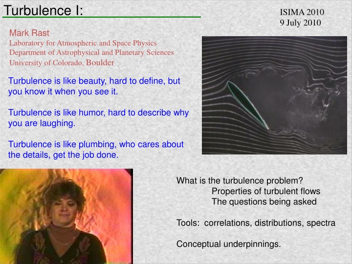
Turbulence I:. ISIMA 2010 9 July 2010. Mark Rast Laboratory for Atmospheric and Space Physics Department of Astrophysical and Planetary Sciences University of Colorado, Boulder. Turbulence is like beauty, hard to define, but you know it when you see it.

E N D
Turbulence I: ISIMA 2010 9 July 2010 Mark Rast Laboratory for Atmospheric and Space Physics Department of Astrophysical and Planetary Sciences University of Colorado, Boulder Turbulence is like beauty, hard to define, but you know it when you see it. Turbulence is like humor, hard to describe why you are laughing. Turbulence is like plumbing, who cares about the details, get the job done. What is the turbulence problem? Properties of turbulent flows The questions being asked Tools: correlations, distributions, spectra Conceptual underpinnings.
Turbulence (3 fundemental properties: random, multi-scale, vortical): • The Navier-Stokes equations are deterministic. Turbulent flows are unpredictable. • Velocity field varies significantly and irregularly in both position and time • Deterministic chaos – hypersensitivity to initial conditions • Nonlinear dynamical system with very large number of degrees of freedom • Importance of nonlinearity depends on Reynolds number Correlation length (integral scale): Dissipation length (Kolmogorov scale): Two-point correlation (instantaneous) Kolmogorov hypothesis: Energy dissipation at small scales = Energy injection at integral scale Fully resolved 3D simulation requires minimum grid points per integral scale Strictly random flow has degrees of freedom. Reduced by correlations within flow (coherent structures).
Multi-scale • Significant energy over many scales – scale separation an idealization • Large scale flow depends on geometry and external forcing • Small scale flow – “universal character” • Period – Scale – Energy relationship: • small scales, high frequency, low energy • large scales, low frequency, high energy Exponential damping with rate fastest at smallest scales. Do triad interactions produce on average ? Werne, Fritts, et al. (1999+) DNS Kelvin-Helmholz instability
Sum of randomly oriented unit vectors in three-dimensions: • Energy transferred in both directions, • but preferentially to smaller scales
Vortical • Turbulence is characterized by high degree of fluctuating vorticity • Kinetic energy density greatest at large scales, Enstrophy at small scales Tilting: exchange between components Stretching: amplification, volume of fluid element constant, radius decreases
Conservation of angular momentum (per unit mass): Vorticity production Energy transfer to small scales Mininni et al. (2006) DNS with Taylor-Green forcing As much destretching as stretching? • Heuristic argument: • random walk – on average the distance • between any two points increases • infinitesimal line elements are on average • stretched by random motions (and folded). Mean enstrophy increases, or maintains itself against viscosity only if On average, there must be a correlation between the magnitude of the vorticity and the gradient of the velocity in the flow. This requires a velocity derivative skewness (NonGaussianity in the derivative statistics).
Goto and Kida (2007) DNS with spectral forcing Turbulent flows characterized by macroscopic mixing to small scales, and thus enhanced microscopic diffusion and dissipation. Two components: Transport – fluid parcels, “mixing” on continuum scale Dissipation – homogenization within/between parcels, transfer to the molecular scale
So what is the Question? What is the turbulence problem? Is there one, or are all flows fundamentally different? High Level: “The problem of turbulence is reduced here [for incompressible flows] to finding the probability distribution P(dω) in the phase space of turbulent flow Ω ={ω}, the points ω of which are all possible solenoidal vector fields u(x,t) which satisfy the equations of fluid mechanics and the boundary conditions imposed at the boundaries of the flow.” The fluid mechanical fields are constrained random fields and every actual example of such a field is a realization of the statistical ensemble of all possible fields. “Thus, in a turbulent flow, the equations of fluid dynamics will determine uniquely the evolution in time of the probability distribution of all the fluid dynamic fields.” – Monin and Yaglom (1971) Splat Spin
Describe the probability distribution in terms of its moments • Truncate the moment expansion to some low order (tractability) • Model the influence of higher order moments (closure) • Evolve low order model Lower Level Description (more explicit low order model): The problem of turbulence is the problem of scalar and vector transport at unresolved scales. Numerical solution of the Navier-Stokes equations can yield a robust realization of the flow at resolved scales, modeling of turbulent transport is needed to bridge the gap between resolved motions and molecular diffusion. What are the characteristics of small-scale turbulent motions, how do these depend on the properties of the large-scale motions from which they derive, and knowing them, how can we model the transport of scalar and vector quantities, such as concentration, energy, or momentum? • Numerical simulation of Navier-Stokes at affordable resolution • Subgrid model of turbulent transport below grid scales
Molecular transport (Maxwell 1866): • Chapman – Enskog: • properly takes into account nonequilibrium • particle distribution functions • due to the presence of the background variations – • transport occurs because (distribution is nonMaxwellian ) Random molecular motions yield – viscosity by the transport of net momentum – conductivity by the transport of net energy – diffusion by the transport of molecular identity Assume (lowest order): Transport of x-momentum: Dynamic Viscosity
Prandtl’s answer (as quoted by Bradshaw 1974) • typical values of the fluctuating velocity components are each proportional to where l is the mixing length (Mischungsweg) • l “may be considered as the diameter of the masses of fluid moving as a whole in each individual case; or again, as the distance traversed by a mass of this type before it becomes blended in with neighboring masses” • l is “somewhat similar, as regards effect, to the mean free path in the kinetic theory of gases” Mixing length theory of turbulent transport (Prandtl 1925): The turbulence problem: How to determine the velocity fluctuations from knowledge of the large scale flow (the closure problem). How to mix – provided by elastic collisions in molecular transport (understanding the interface between continuum and molecular dynamics) Two meanings of the mixing length Shear stress: Turbulent viscosity:
If turbulent motions were strictly random, turbulent viscosity would be proportional the average magnitude of the velocity perturbations – It is the coherent motions that are key, phase relations are critical • Turbulent transport requires a “mixing length” – turbulent mean free path – Must understand the interface between continuum and molecular dynamics to understand where in the flow the transported quantity is deposited Formulate a statistical description of turbulent coherent structures, Lagrangian dynamics in their presence, and mixing between parcels
Tools to describe hydrodynamic fields treated as continuous random variables • probability density functions – distributions of values in occurrence • spatial correlations – distribution of values in physical space • power spectra – distribution of values in spectral space Probability density function: • Hydrodynamic fields are described by a joint probability density function for all (x,t) • Moments completely determine distribution • Navier-Stokes provide constraints on evolution of PDFs with moments: Mean: Variance: Skewness: Flatness:
Gaussian distribution: All moments can be expressed in terms of mean and variance Central Limit Theorem: Let X1, X2, X3, …, Xnbe a sequence of nindependent and identically distributed random variables with finite mean μ and variance σ2. As the sample size increases the distribution of the sample average of these random variables approaches the normal distribution with mean μ and variance σ2/n, independent of the underlying common distribution. The sum of a large number of identically distributed independent variables has a Gaussian probability density, regardless of the shape of the pdf of the variables themselves. • In general probability density functions of turbulent fields are nonGaussian • velocity generally slightly subGaussian • velocity difference (increment) significantly superGaussian (intermitancy) – elevated extremes Mordant, Leveque, & Pinton (2004)
Mininni et al. (2008+): Forced turbulence (Taylor-Green) at resolution of 10243 Forcing scale 2π/kf , kf =2
What are these PDFs, what should they be? What are they supposed to represent? The treatment of turbulent motions statistically, via random variables, means that the flow can only be considered as a statistical ensemble of realizations characterized as by some jont probability density for the values of all fluid dynamic variables. The moments are the expectation values (e.g. ensemble means or probability means) of the flow over many realizations. In practice, averaging over multiple realizations is replaced by spatial or temporal averaging (the ergodic theorem). Not independent random variables, coupled by Navier–Stokes
if its statistical properties (such as its mean and variance) can be deduced from a single, sufficiently long sample (realization) of the process Ergodicity: For stationary random process and time-averaging (or homogeneous random field and spatial-averaging) Necessary and sufficient condition for quadratic convergence to the ensemble mean U Experiment Number is that the two-point correlation (autocovariance) satisfies: Velocity fluctuations de-correlate in time (or space). The integral time scale (correlation time): Ergodic if integral time scale is finite, use averaging time T >T1.
Moment equations (Navier-Stokes constraints on evolution of distributions): Lowest order (the Reynolds average equations): Decompose fields into sum of their mean and fluctuations: Note: Note: Take the Average of each term (averages of fluctuations vanish, ensemble averaging commutes with differentiation): Reynolds stresses link orders (the closure problem) Reynolds stresses act like viscosity
Closure problem: Full Navier-Stokes minus Reynolds average equation yields: Multiplying by and averaging to obtain an equation for (e.g. Hinze1959), an evolution equation for the Reynolds stresses, yields new unknowns: • third-order central moments • multiples by ν of second-order moments and their spatial derivatives • third and second moments of pressure and velocity products none of which can be expressed directly in terms of Reynolds stresses. The equations are not truncate-able or perhaps tractable: At each step the difference between the number of unknowns and the number of equations increases. The Friedman-Keller equations (Keller and Friedmann 1924) are an infinite chain of coupled moment equations. M.C. Esher, Snakes, 1969 woodcut
Modeling the Reynolds stresses: Divergence of momentum flux by molecular motions and velocity fluctuations (mixing – moving and averaging) Momentum change in volume due to flow: Advection Mean ith component: Similarly the scalar transport equation: can be written in terms of mean and fluctuating components suggesting an enhanced diffusive flux
Down gradient diffusion model (turbulence mimics molecular transport): Scalar turbulent diffusivity, so that: with Turbulent transport analogous to Fick’s law of molecular diffusion. Molecular transport of momentum (surface forces on parcel of a Newtonian fluid): Stress tensor has both static isotropic (independent of surface orientation) and deviatoric (due to fluid motion) components Linear relationship between stress and strain rate. Stokes assumption (only translational degrees of freedom – monatomic ideal gas) Down gradient momentum flux
Turbulent transport by analogy: Scalar turbulent viscosity (Boussinesq 1877), so that deviatoric Reynolds stress tensor is proportional to the mean rate of strain: Normal stresses (twice the turbulent kinetic energy k) Shear stresses Isotropic component (turbulent pressure) deviatoric component (turbulent viscosity) Incompressible Navier-Stokes with “eddy viscosity” and modified mean pressure. Specify νT solves closure problem (second-order closure model), eliptical problem for pressure solves for total pressure not gas. Note:
Turbulence must be vortical for turbulent shear stresses to exist: Consider random incompressible irrotational flow: (Corrsin and Kistler 1954) In an irrotational flow, shear stresses have same effect as isotropic stresses – can be absorbed into a modified pressure and have no effect on mean flow. In a simple shear flow (mean gradients perpendicular to mean flow), the assumed Reynolds stress / mean gradient relationship becomes a definition of the turbulent-viscosity: Single covariance related to a single mean gradient.
local stress / rate of strain relationship: • Non-local transport processes invalidate the hypothesized relationship • between turbulent Reynolds stress and the local mean gradients • Model works best when production and dissipation of turbulent kinetic energy • are approximately in balance, Axisymmetric contraction experiment: Reynolds stress anisotropies produced in contraction (extensive axial and compressive lateral strain) are advected downstream and influence the mean flow in a way not described by mean rate of strain. Reynolds stresses reflect history not local mean rates of strain. Statistical state of molecular motion adjusts rapidly to imposed shearing Kinetic theory: Simple shear flow timescale: Turbulence decay rate: Statistical state of turbulent motions adjusts slowly to imposed shearing Turbulence does not adjust rapidly enough to imposed mean straining – no general basis for local stress / rate of strain relationship.
Models of the turbulent viscosity (νT): The turbulent viscosity is the product of a velocity and a length: I. Mixing-length model: (simple shear flow) Clearly not correct for decaying grid turbulence, centerline of round jet, etc. where mean velocity gradient is zero but the turbulent velocity scale is not. II. Kolmogorov-Prandtl model: Need: Must solve model transport equation for k(x,t) – called a one-equation model: • Strategy: • specify mixing length • solve model equation for k • turbulent viscosity hypothesis • Solve RANS for
Equation for k(turbulent kinetic energy ): Closure Approximations Down gradient flux of turbulent kinetic energy Flux: Production: Turbulent viscosity hypothesis Dissipation: Kolmogorov hypothesis: Energy dissipation at small scales = Energy injection at integral scale Note: Close form, BUT fundamentally incomplete – mixing length lm must be specified.
III. k – ε model (two-equation model): • model transport equations for two turbulence quantities (in this case k and ε) • can be complete (constants, but flow dependent quantities (like lm) are not required). Model transport equation for k (same as that in one-equation model) Model transport equation for ε (empirical, RANS equation for ε describes processes in dissipative range) Specify turbulent viscosity as (depends only on turbulence quantities, independent of mean flow properties) Standard values! (Launder and Sharma 1974) • the simplest complete turbulence model • incorporated into many commercial CFD codes • has been applied to a wide range of incompressible flows and, modified, to a more limited • range of compressible problems • inaccuracies stem from the underlying turbulent viscosity hypothesis and from the ε equation • ε equation and constants can be obtained via renormalization group methods
Beyond RANS models: PDF methods: • The mean velocity and Reynolds stresses are only the first and second moments of the Eulerian velocity PDF . • PDF methods evolve an exact, but unclosed, equation for the evolution of the one point, one time Eulerian PDF of the velocity , derived from incompressible Navier–Stokes. Pope, S.B. (2008), Turbulent Flows Dopozo, C. (1994), Recent developments in PDF methods, in Turbulent Reacting Flows O’Brien, E.E. (1979), The probability density function (pdf) approach to reacting turbulent flows, in Topics in Applied Physics, Vol. 44
Spatial correlations and the velocity power spectrum: Two point correlation (two-point, one-time covariance): For homogeneous turbulence: Fourier transform: And its inverse: Autocorrelation theorem: the power spectrum of a function is the Fourier transform of its autocorrelation For : Define: Integrate over shell: spectral kinetic energy density per unit mass – contribution to kinetic energy by modes with wavenumbers between kand k+dk
Kolmogorov (1941): • Inertial range: energy neither injected or dissipated. In a steady state, energy at any size scale depends only on injection/dissipation rate and size scale, not viscosity -- spectral slope by dimensional analysis local energy flux • Energy is injected a the integral scales: energy injection rate • Disipative scales: Energy is removed at the same rate it is injected
Fluid instabilities produces ever smaller scales from large scale motions • Big whirls have little whirls, which feed on velocity; and little whirls have lesser whirls, and • so on to viscosity (in the molecular sense). (Richardson 1922 after Jonathan Swift) Spectra: all phase information lost model of transport in spectral space Transport in physical space? Formulate a statistical description of turbulent coherent structures, Lagrangian dynamics in their presence, and mixing between parcels