Download
1 / 31
310 likes | 425 Views
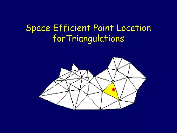
Space Efficient Point Location forTriangulations. Inspiration:. Graphics software wants to light a model and needs to know which face a light ray hits You moved the mouse and the windowing system would like to know which window has focus now.

E N D
Inspiration: • Graphics software wants to light a model and needs to know which face a light ray hits • You moved the mouse and the windowing system would like to know which window has focus now. • Given latitude and longitude you need to determine which country/city/neighborhood contains your destination
The problem at hand • Input: • 1) A set of n unlabeled points in R2 (beforehand) • 2) Additional points called query points • The task: • Create a triangulation using the initial set of points as an offline preprocessing step. Then for each query point, return the triangle which contains it. • And make the data fit in O(n) bits • (not including storage of the n input points) • with query times of O(log n).
In order to accomplish the task we will use a combination of algorithms. • A point location algorithm which uses O(log n) time • and O(n log n) space. • - Edelsbrunner, Guibas, Stolfi 84 • 2) “Edgebreaker” with “Wrap&Zip” • A compression algorithm for triangulations which operates in O(n) time and compresses to O(n) space. • - King and Rossignac 99 • - Rossignac and Szymczak 99 • (In fact either algorithm can be replaced with others, but this is at least an interesting sample solution)
Separators The key of the point location algorithm is a recursive subdivision of the triangulation using a subset of line segments and vertices which span from left to right. We call this a separator.
Separators This algorithm actually works on any planar graph in which each vertex has at least one edge to the left and right. Adding extra edges outside the boundary during pre-processing will let our triangulation have this property too.
Separators For now we will simply take for granted that is possible to repeatedly divide the triangulation until only single triangles remain. The details of how to best pick separators are not too important.
Separator-Tree By placing all the separators into a binary tree, a simple binary search gives point location. Test the point to see if it is above or below each separator while descending the tree.
Separator-Tree search algorithm To test a point against a separator 1) binary search the x-coordinates. 2) Line side test against the segment Since that may take O(log n) time and there will be O(log n) separators to test against this yields an O(log2 n) algorithm.
Improving the Separator-Tree search algorithm If each separator has O(n) edges in it and we need n separators then space usage will be O(n2 log n). We need to lower space usage. Also every time we descended to the next level in the separator tree all the x-coordinate information was lost. We need to be able to find the proper segment of the next separator with only O(1) rather than O(log n) extra effort.
Improving the space usage to O(n log n) It is possible to store each edge only once. For each edge determine the subset of separators which contain it and then find the least common ancestor (LCA) in the binary tree. This LCA will also contain that edge (not proved here). Each of these circled edges is identical
Improving the space usage to O(n log n) Rather than re-encode the edge we place a gap. The total number of gaps and edges will be O(n). Many edges can coalesce into one gap
Improving the running time Add pointers between segments of the parent and child which overlap vertically. Now only need to search a subset of the child segments
Improving the running time But we may still have to look at too many child segments! This will not improve the worst case run time
Improving the running time By further subdividing edges (or gaps) we can ensure that a parent segment vertically overlaps at most 2 child segments. This subdivision also only increases the total number of edges and gaps by a constant factor
Edelbrunner et al. point location algorithm What we have covered so far represents the original point location algorithm. With some additional optimizations it can be made into an O(log m) time and O(n + m log m) space algorithm, where m represents the number of regions in the graph (and n is still points).
The main idea from here We will use this algorithm on only O(n/log n) of the original regions. If we can then compress small regions of O(log n) triangles we can decompress and search them in only O(log n) time while using only O(n) total space.
How to sub-sample All that needs be done is too stop the subdivision process at regions of size between log n and 2 log n triangles. It can be made to preserve contiguous triangulated regions.
How to sub-sample Again we could do it entirely differently…. A known result in this area is that any planar graph can be divided with trapezoids. It takes O(r) trapezoids to ensure each trapezoid intersects at most r/n line segments. Letting r = n / log n produces another top level sampling on which any O(n log n) space algorithm could be used.
Compression All that is required for a compression algorithm is that it has O(n) time decompression and can store a graph in O(n) bits. While many types of graphs have algorithms which can do this, triangulations have an interesting one… (Alternatively some graph compression formats can be traversed in O(n) time without needing a decompression step, that works too)
Edgebreaker This algorithm encodes a triangulation as a string of {C,L,E,R,S} characters while performing a depth first search of the triangulation. A worst case encoding is guaranteed not to use more than 1.84 bits per vertex. This is only 13% over the information-theoretic bound. CCRCL….
Edgebreaker – How it works… The algorithm performs a depth first search of the triangulation, encoding each triangle with one of the characters. Which character depends on whether or not adjacent triangles/vertices have been visited. A vertex is considered visited if it is adjacent to a triangle that is visited.
Edgebreaker – How it works… The bottom triangle is the one previously encoded, the middle triangle is currently being encoded. Red triangles/vertices have already been visited, white ones have not. The arrow shows where to go next. C L R
Edgebreaker – How it works… These operations require a stack and represent the branches and terminal leaves of a tree traversal. Push left triangle Pop next triangle S E
Wrap and Zip – How it works… Decompression works by first generating a tree of adjacent triangles. Then the free edges of triangles are given an orientation (wrapping). Finally similarly oriented edges are joined (zipping). How to Wrap: C L E R S
Wrap and Zip – How it works… How to Zip: Vertices with adjacent edges pointing inwards should merge those edges. Repeat until all edges are zipped.
Putting it all together To create our final data structure, run the point location pre-process until it reaches regions of size less than c log n. Then encode those regions using Edgebreaker. The top level structure has size O(n) and all of the Edgebreaker encodings have size O(log n) * n/clog n regions, giving O(n) total size. CCLR…
Putting it all together To search in the structure first search in the high level structure then decompress the resulting small region and search through it using brute force. The top level search uses O(log n) time, the decompression and brute force search on the small region is also O(log n).
Putting it all together While I have yet to implement this algorithm, it seems that the constants present are also good. However it is not overly simple once all the bells and whistles are in place. I am continuing to search out some good alternates. I believe there is a decent chance it will be more compact than any of the existing low space solutions even with small data sets.
Putting it all together On issues of time, typically these algorithms are judged solely on the number of line-side tests. This algorithm uses (2+ε) log n tests at most, whereas the fastest known uses log n + 2 sqrt(log n). The fastest O(n log n) space algorithms use 2 log n tests. Nonetheless the decompression step likely makes this comparison less accurate at measuring the run-time constants.
Going further Very little is dependent upon having a triangulated graph. Using different compression techniques would allow this to work on any planar graph. A sample implementation is also needed to gather data to do a more practical comparison with alternative O(n) space solutions.