V11: Folding of Membrane Proteins

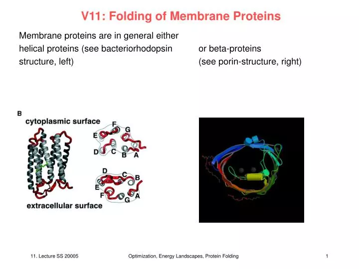
1. V11: Folding of Membrane Proteins Membrane proteins are in general either helical proteins (see bacteriorhodopsin or beta-proteins structure, left) (see porin-structure, right) Optimization, Energy Landscapes, Protein Folding

2. Folding of helical membrane proteins Paradigm by Engelman & Popot: 2-step mechanism (i) -helices fold after being inserted into membrane (ii) folded -helices then assemble to form entire protein Today‘s program: 1 recent discoveries on translocon-mediated insertion into lipid bilayer. 2 apply protein engineering to helix-connecting loops in bR  kinetics 3 rupture individual bR proteins out of membrane by atomic force microscopy Optimization, Energy Landscapes, Protein Folding

3. Folding of helical membrane proteins (II) White, FEBS Lett. 555, 116 (2003) Optimization, Energy Landscapes, Protein Folding

4. Hydrophobicity Scales White, FEBS Lett. 555, 116 (2003) Optimization, Energy Landscapes, Protein Folding

5. Translocon-assisted folding of TM proteins? Upper picture (model!): the newly synthesized polypeptide chain of a membrane protein is inserted from the ribosome into the membrane via interaction with a TM complex, the “translocon” (EM map shown). lower picture: experiment largely supports the concerted view. What determines insertion into the membrane ? White, FEBS Lett. 555, 116 (2003) Optimization, Energy Landscapes, Protein Folding

6. Integration of H-segments into the microsomal membrane Ingenious experiment! Introduce marker that shows whether helix segment H is inserted into membrane or not. a, Wild-type Lep has two N-terminal TM segments (TM1 and TM2) and a large luminal domain (P2). H-segments were inserted between residues 226 and 253 in the P2-domain. Glycosylation acceptor sites (G1 and G2) were placed in positions 96–98 and 258–260, flanking the H-segment. For H-segments that integrate into the membrane, only the G1 site is glycosylated (left), whereas both the G1 and G2 sites are glycosylated for H-segments that do not integrate in the membrane (right). b, Membrane integration of H-segments with the Leu/Ala composition 2L/17A, 3L/16A and 4L/15A. Bands of unglycosylated protein are indicated by a white dot; singly and doubly glycosylated proteins are indicated by one and two black dots, respectively. Hessa et al., Nature 433, 377 (2005) Optimization, Energy Landscapes, Protein Folding

7. Insertion determined by simple physical chemistry measure fraction of singly glycosylated (f1g) vs. doubly glycosylated (f2g) Lep molecules c, Gapp values for H-segments with 2–4 Leu residues. Individual points for a given n show Gapp values obtained when the position of Leu is changed. d, Mean probability of insertion (p) for H-segments with n = 0–7 Leu residues. Hessa et al., Nature 433, 377 (2005) Optimization, Energy Landscapes, Protein Folding

8. Biological and biophysical Gaa scales a, Gappaa scale derived from H-segments with the indicated amino acid placed in the middle of the 19-residue hydrophobic stretch. Only Ile, Leu, Phe, Val really favor membrane insertion. All polar and charged ones are very unfavored. b, Correlation between Gappaa values measured in vivo and in vitro. c, Correlation between the Gappaa and the Wimley–White water/octanol free energy scale for partitioning of peptides. Hessa et al., Nature 433, 377 (2005) Optimization, Energy Landscapes, Protein Folding

9. Positional dependencies in Gapp Tyr and Trp are favorable in interface region. a, Symmetrical H-segment scans with pairs of Leu (red), Phe (green), Trp (pink) or Tyr (light blue) residues. The Leu scan is based on symmetrical 3L/16A H-segments with a Leu-Leu separation of one residue (sequence shown at the top; the two red Leu residues are moved symmetrically outwards) up to a separation of 17 residues. For the Phe scan, the composition of the central 19-residues of the H-segments is 2F/1L/16A, for the Trp scan it is 2W/2L/15A, and for the Tyr scan it is 2Y/3L/14A. The G app value for the 4L/15A H-segment GGPGAAALAALAAAAALAALAAAGPGG is also shown (dark blue). b, Red lines show G app values for symmetrical scans of 2L/17A (triangles), 3L/16A (circles), and 4L/15A (squares) H-segments. c, Same as b but for a symmetrical scan with pairs of Ser residues in H-segments with the composition 2S/4L/13A. Hessa et al., Nature 433, 377 (2005) Optimization, Energy Landscapes, Protein Folding

10. Folding kinetics of bR Fluorescence: bO  I1  I2  IR  bR bO: denatured bR in SDS (4 TM helices) I1: fastest kinetic phase after mixing of SDS and DHPC/DMPC micelles, 4 – 10 ms, increase in fluorescence I2: important folding intermediate, another 1.25 TM helices form (CD) Allen et al. J Mol Biol 308, 423 (2001) Optimization, Energy Landscapes, Protein Folding

11. What effect do the loops have on folding kinetics of bR? Scheme shows which loops were replaced by structureless linkers of Gly-Gly-Ser repeats. The loops were replaced in turn by linkers of the same length as the wild-type loop. Linkers of two different lengths were used to replace the BC loop: one shorter than the wild-type loop (BC1) and one the same length as the wild-type loop (BC3). Allen et al. J Mol Biol 308, 423 (2001) Optimization, Energy Landscapes, Protein Folding

12. Kinetics of formation of native-like chromophore for wt and loop mutants (a) Kinetic spectra for the two time constants resolved in time-resolved absorption studies during folding of wild-type ebO to bR, showing the wavelength-dependence of the amplitude of the 130 seconds and 4180 seconds components. (b) Changes in 560 nm absorbance during folding of ebO, AB, CD and EF loop mutants and at 500 nm for BC1 mutant. (c) Changes in 560 nm absorbance during folding of ebO and the DE loop mutant and at 541 nm for the FG mutant. Allen et al. J Mol Biol 308, 423 (2001) Optimization, Energy Landscapes, Protein Folding

13. Effects of loop mutants on folding kinetics Mutation of CD or EF loops shows slower apoprotein folding to I2 mutation of FG loop shows slower rate of the events accompanying retinal binding to the protein. Allen et al. J Mol Biol 308, 423 (2001) Optimization, Energy Landscapes, Protein Folding

14. AFM topography of a purple membrane Typical high-resolution AFM topograph of the cytoplasmic surface of a wild-type purple membrane. BR assembles in trimers that arrange in a hexagonal lattice. To catch an individual protein (white circle), we zoomed in by reducing the frame size and the number of pixels. After the AFM tip was positioned, it was kept in contact with the selected protein for about 1 s while a force of ~1 nN was applied to give the protein the chance to adsorb on the stylus. In 15% of the cases, the protein can then be extracted. Oesterhelt, F et al. Science 288, 143 (2000) Optimization, Energy Landscapes, Protein Folding

15. Force profile The stylus and protein surface were separated at a velocity of 40 nm/s while the force spectrum was recorded. The interaction between tip and surface, which is expressed in the marked discontinuous changes in the force, indicates a molecular bridge between tip and sample. This bridge reaches far out to distances up to 75 nm, which corresponds to the length of one totally unfolded protein. Oesterhelt, F et al. Science 288, 143 (2000) Optimization, Energy Landscapes, Protein Folding

16. Check membrane to see what happened After the adhesive force peaks were recorded, a topograph of the same surface was taken to show structural changes. Note that a single monomer is missing. Thus, the recorded force spectrum may be correlated to extraction of an individual protein from the membrane. Oesterhelt, F et al. Science 288, 143 (2000) Optimization, Energy Landscapes, Protein Folding

17. Force extraction profiles Several force spectra taken on wild-type BR are shown. A typical repeating pattern is visible. All curves show four peaks located around 10, 30, 50, and 70 nm. Oesterhelt, F et al. Science 288, 143 (2000) Optimization, Energy Landscapes, Protein Folding

18. What are the regular features? Thirteen spectra are superposed on the second peak. This results in an exact cover of the third and fourth peaks, whereas the first peak remains scattered. Gray lines are force extension curves calculated by the worm-like chain model with a Kuhnlength of 0.8 nm, which is known to describe the elasticity of an unfolded poly-amino acid chain. Oesterhelt, F et al. Science 288, 143 (2000) Optimization, Energy Landscapes, Protein Folding

19. Model to explain force extraction spectra This model explains the peaks in the force spectra as the sequential extraction and unfolding of a single BR. A rupture length of more than 60 nm can be recorded only if the COOH-terminus has adsorbed on the tip. If a force is applied on the COOH-terminus, helices F and G will be pulled out of the membrane and unfold. Upon further retraction, the unfolded chain will be stretched and a force will be applied on helices D and E until they are extracted from the membrane. Thus, peak 2 reflects unfolding of helices D and E and peak 3 reflects unfolding of helices B and C. Peak 4 shows extraction of the last remaining helix A. Oesterhelt, F et al. Science 288, 143 (2000) Optimization, Energy Landscapes, Protein Folding

20. 3-dimensional structure of bR (A) BR is a 248-amino acid membrane protein that consists of seven transmembrane -helices, which are connected by loops. (B) Three-dimensional model and top and bottom view show spatial arrangement of the helices. Helices F and G are neighboring helices A and B and thus can stabilize them. Oesterhelt, F et al. Science 288, 143 (2000) Optimization, Energy Landscapes, Protein Folding

21. How to check correctness of model? Mutations! Force curves were recorded on BR where the E-F loop was cleaved enzymatically. (A) Selection of the longest force curves taken on the cleaved BR. No recorded spectrum showed a rupture length beyond 50 nm. Only three main peaks are visible-around 5, 25, and 45 nm--and the second is a double peak. (B) Superposition of 17 spectra on the second peak results in an exact cover of all but the first peak. (C) Because loop F-G is cut out, force curves with a length of 45 nm can be recorded only when the free end of helix E is fixed to the tip. Thus, the first peak reflects extraction of helices D and E and the second reflects extraction and unfolding of helices B and C; the last peak shows extraction of the last remaining helix A. Consequently, the intermediate peak between peaks 2 and 3 reflects stepwise unfolding of helices A and B. Oesterhelt, F et al. Science 288, 143 (2000) Optimization, Energy Landscapes, Protein Folding

22. bR mutant G241C with specific anchoring of COOH-terminus (A) Force spectra of G241C where a terminal cysteine was introduced near the COOH-terminus at position 241, allowing specific attachment to a gold evaporated tip. In these experiments, the percentage of full-length force curves increased to 80%. (B) Thirty-five force curves are superposed and WLC fits with lengths corresponding to the model shown in Fig. 2 are drawn. In contrast to the measurements in which we used unspecific attachment, we also could resolve the substructure of the first peak, which reflects unfolding of helices F and G. Oesterhelt, F et al. Science 288, 143 (2000) Optimization, Energy Landscapes, Protein Folding

23. Unfolding bR from purple membrane at various temperatures (A ) Force curves of individual BR molecules recorded at 25°C. To show common unfolding patterns among single-molecule events, the force spectra recorded at different temperatures were superimposed. (B–F) BR unfolded at different temperatures. Required pulling forces are smaller are higher temperatures! Janovjak et al. EMBO J. 22, 5220 (2003) Optimization, Energy Landscapes, Protein Folding

24. Unfolding pathways of bR Janovjak et al. EMBO J. 22, 5220 (2003) (A–D) Unfolding events of individual secondary structures. (A) Occasionally the first major unfolding peak shows side peaks at about 26, 36 and 51 aa. The peak at 26 aa indicates the unfolding of the cytoplasmic half of helix G up to the covalently bound retinal, which is embedded in the hydrophobic membrane core. The peak at 36 aa indicates the G helix to be unfolded completely. At 51 aa, helix G and the loop connecting helices G and F are unfolded and the force pulls directly on helix F until this helix unfolds together with loop EF. (B) The side peaks of the second major peak indicate the stepwise unfolding of helices E and D and loop DE. The peak at 88 aa indicates the unfolding of helix E, that at 94 aa of the loop DE, and the peak at 105 aa indicates unfolding of helix D. (C) The side peaks of the third major peak indicate the stepwise unfolding of helices C and B and loop BC. The peak at 148 aa indicates the unfolding of helix C, that at 158 aa of the loop BC, and the peak at 175 aa indicates unfolding of helix B. (D) The side peak of the last major peak indicates the unfolding of helix A (219 aa) and of the pulling of the N-terminal end through the purple membrane (232 aa). Optimization, Energy Landscapes, Protein Folding

25. Unfolding of individual secondary structure elements (A) Occasionally the first unfolding peak at 88 aa shows two shoulder peaks, which indicate the stepwise unfolding of the helical pair. If both shoulders occur, the peak at 88 aa indicates the unfolding of helix E, that at 94 aa of loop DE, and the peak at 105 aa corresponds to the unfolding of helix D. (B) The shoulder peaks of the second peak indicate the stepwise unfolding of helices C and B and loop BC. The peak at 148 aa indicates the unfolding of helix C, that at 158 aa of the loop BC, and the peak at 175 aa represents unfolding of helix B. The arrows indicate the observed unfolding pathways. In certain pathways (black arrows), a pair of two transmembrane helices and their connecting loop unfolded in a single step. In other unfolding pathways (colored arrows), these structural elements unfolded in several intermediate steps. Janovjak et al. Structure 12, 871 (2004) Optimization, Energy Landscapes, Protein Folding

26. Unfolding forces of secondary structure elements depend on temperature (A) Rupture forces of main peaks, which exhibited no side peaks. The forces represent the pairwise unfolding of transmembrane helices E and D (88 aa), C and B (148 aa) and the unfolding of helix A (219 aa). (B–D) Rupture forces of side peaks represent unfolding of single -helices and of their connecting loops (see text). The thermally induced weakening of the unfolding forces was fitted (dotted lines) using equation (2). Janovjak et al. EMBO J. 22, 5220 (2003) Optimization, Energy Landscapes, Protein Folding

27. Probability of unfolding pathways depends on temperature Janovjak et al. EMBO J. 22, 5220 (2003) • The occurrence of main force peaks exhibiting no side peaks (solid lines) increased with increasing temperature. As a consequence, the probability of the main peaks exhibiting side peaks (dashed lines) decreased significantly. • -helices of BR unfold preferentially pairwise at elevated temperatures. The probability of single structural elements, such as helices or loops, to unfold in a separate event decreases with increasing temperature. Optimization, Energy Landscapes, Protein Folding

28. 2-state model to interpret mechanical unfolding experiments A simple two-state potential exhibiting a single sharp potential barrier separating the folded low-energy state (F) from the unfolded state (U) can be applied to describe the mechanical unfolding experiments. Here the unfolding of single secondary structure elements of the membrane protein BR is interpreted using this model. The activation energy for unfolding is given by ΔG‡u, while xu (the width of the potential barrier) is the distance along the reaction coordinate from the folded state to the transition state (‡) and the natural (thermal) transition rate is denoted k0u . DFS experiments allow determining the width of the potential barrier and the unfolding rate by monitoring the unfolding forces as a function of pulling speed. Janovjak et al. Structure 12, 871 (2004) Optimization, Energy Landscapes, Protein Folding

29. bR force curves recorded at different pulling velocities (A)–(D) show superimpositions of around 15 force versus distance traces each recorded on a single BR molecule at the pulling speed indicated (10 nm/s [A], 87 nm/s [B], 654 nm/s [C], 1310 nm/s [D], and 5230 nm/s [E]). As observed from the superimpositions, the unfolding forces (height of the peaks) increase with the pulling speed. Janovjak et al. Structure 12, 871 (2004) Optimization, Energy Landscapes, Protein Folding

30. Pairwise unfolding pathway of TM helices The experimental curve to the left shows a representative unfolding spectrum of a single BR, while the schematic unfolding pathway is sketched on the right. The worm-like chain model was applied to derive the length of the unfolded elements based on their force-extension pattern (solid lines). These lengths were then used to reconstruct the corresponding unfolding pathway. The first force peaks detected at tip-sample separations below 15 nm indicate the unfolding of transmembrane α helices F and G. After unfolding these elements, 88 aa are tethered between the tip and the surface (a). Separating the tip further from the surface stretches the polypeptide (b), thereby exerting force to helix E and D. At a certain critical load, the mechanical stability of helices E and D is overcome and they unfold together with loop DE. As the number of amino acids linking the tip and the surface is now increased to 148, the cantilever relaxes (c). In a next step, the 148 aa are extended thereby pulling on helix C (d). After unfolding helices B and C and loop BC in a single step, the molecular bridge is lengthened to 219 aa (e). By further separating tip and purple membrane, helix A unfolds (f) and the polypeptide is completely extracted from the membrane (g). Janovjak et al. Structure 12, 871 (2004) Optimization, Energy Landscapes, Protein Folding

31. Unfolding Forces as a Function of Pulling Speed For single and groups of secondary structure elements, the unfolding force increased with the pulling speed. A logarithmic dependence of the force on the pulling speed was clearly resolved. This indicated that a single sharp potential barrier as shown in Figure 1 was to be crossed to unfold the structural elements. Force versus ln(speed) plots for the pairwise unfolding of helices are shown in (A) and for single secondary structure elements (i.e., transmembrane α helices and polypeptide loops) in (B)–(F). As unfolding of helices D, C, and B occurred in two different unfolding pathways (1 and 2), two data sets were obtained and analyzed independently. Although in both pathways these helices unfolded individually, other helices unfolded together with extracellular loops, and therefore the events were analyzed separately. Janovjak et al. Structure 12, 871 (2004) Optimization, Energy Landscapes, Protein Folding

32. Unfolding Pathways Depend on Pulling Speed Janovjak et al. Structure 12, 871 (2004) Individual bR molecules exhibited distinct probabilities to follow different unfolding pathways when unfolded by mechanically pulling on the C terminus. Although single helices were sufficiently stable to unfold in individual steps (dashed lines), they exhibited a certain probability to unfold pairwise (solid lines). Changing the pulling speed affected these unfolding probabilities: the probability of unfolding single secondary structure elements increased with the pulling speed. This suggests that in the absence of a pulling force (smallest pulling speeds) two transmembrane helices would preferentially show a pairwise behavior. Optimization, Energy Landscapes, Protein Folding

33. Potential Landscape from Dynamic Force Spectroscopy Two possible unfolding routes exist for pairs of transmembrane helices in BR. From the folded state (F), the two helices are either unfolded individually (dashed line) or pairwise (solid line) to the unfolded state (U ). The shown approximation of the potential landscape at native conditions (zero force) was generated by extrapolating the speed-dependent unfolding probabilities to zero force. Since the experimental data showed that between two possible routes the pairwise unfolding was chosen more frequently, its potential barrier must be lower than for unfolding of individual helices. Janovjak et al. Structure 12, 871 (2004) Optimization, Energy Landscapes, Protein Folding

34. Summary 2-step mechanism suggested by Engelman & Popot 1) -helices fold first after being inserted into membrane 2) folded -helices then assemble to form entire protein is well supported by recent experiments. Translocon complex inserts TM helices into lipid bilayer. Fluorescence allows to follow folding events upon denaturation/renaturation. AFM experiments allow to study cooperativity of unfolding of secondary structure elements. Remains: integrate these results + combine with simulations. Optimization, Energy Landscapes, Protein Folding