Download
1 / 80
810 likes | 844 Views
Hamiltonian Formalism. Adrien-Marie Legendre (1752 –1833). Legendre transformations Legendre transformation :. What is H? Conjugate momentum Then So. What is H?. What is H?. What is H? If Then Kinetic energy In generalized coordinates. What is H?

E N D
Adrien-Marie Legendre (1752 –1833) • Legendre transformations • Legendre transformation:
What is H? • Conjugate momentum • Then • So
What is H? • If • Then • Kinetic energy • In generalized coordinates
What is H? • For scleronomous generalized coordinates • Then • If
What is H? • For scleronomous generalized coordinates, H is a total mechanical energy of the system (even if H depends explicitly on time) • If H does not depend explicitly on time, it is a constant of motion (even if is not a total mechanical energy) • In all other cases, H is neither a total mechanical energy, nor a constant of motion
Sir William Rowan Hamilton (1805 – 1865) • Hamilton’s equations • Hamiltonian: • Hamilton’s equations of motion:
Hamiltonian formalism • For a system with M degrees of freedom, we have 2M independent variables q and p: 2M-dimensional phase space (vs. configuration space in Lagrangian formalism) • Instead of M second-order differential equations in the Lagrangian formalism we work with 2M first-order differential equations in the Hamiltonian formalism • Hamiltonian approach works best for closed holonomic systems • Hamiltonian approach is particularly useful in quantum mechanics, statistical physics, nonlinear physics, perturbation theory
Hamilton’s equations in symplectic notation • Construct a column matrix (vector) with 2M elements • Then • Construct a 2Mx2M square matrix as follows:
Hamilton’s equations in symplectic notation • Then the equations of motion will look compact in the symplectic (matrix) notation: • Example (M = 2):
Lagrangian to Hamiltonian • Obtain conjugate momenta from a Lagrangian • Write a Hamiltonian • Obtain from • Plug into the Hamiltonian to make it a function of coordinates, momenta, and time
Lagrangian to Hamiltonian • For a Lagrangian quadratic in generalized velocities • Write a symplectic notation: • Then a Hamiltonian • Conjugate momenta
Lagrangian to Hamiltonian • Inverting this equation • Then a Hamiltonian
Hamilton’s equations from the variational principle • Action functional : • Variations in the phase space :
Hamilton’s equations from the variational principle • Integrating by parts
Hamilton’s equations from the variational principle • For arbitrary independent variations
Conservation laws • If a Hamiltonian does not depend on a certain coordinate explicitly (cyclic), the corresponding conjugate momentum is a constant of motion • If a Hamiltonian does not depend on a certain conjugate momentum explicitly (cyclic), the corresponding coordinate is a constant of motion • If a Hamiltonian does not depend on time explicitly, this Hamiltonian is a constant of motion
Higher-derivative Lagrangians • Let us recall: • Lagrangians with i > 1 occur in many systems and theories: • Non-relativistic classical radiating charged particle (see Jackson) • Dirac’s relativistic generalization of that • Nonlinear dynamics • Cosmology • String theory • Etc.
Mikhail Vasilievich Ostrogradsky (1801 - 1862) • Higher-derivative Lagrangians • For simplicity, consider a 1D case: • Variation
Higher-derivative Lagrangians • Generalized coordinates/momenta:
Higher-derivative Lagrangians • Euler-Lagrange equations: • We have formulated a ‘higher-order’ Lagrangian formalism • What kind of behavior does it produce?
Example • H is conserved and it generates evolution – it is a Hamiltonian! • Hamiltonian linear in momentum?!?!?! • No low boundary on the total energy – lack of ground state!!! • Produces ‘runaway’ solutions: the system becomes highly unstable - collapse and explosion at the same time
‘Runaway’ solutions • Unrestricted low boundary of the total energy produces instabilities • Additionally, we generate new degrees of freedom, which require introduction of additional (originally unknown) initial conditions for them • These problems are solved by means of introduction of constraints • Constraints restrict unstable behavior and eliminate unnecessary new degrees of freedom
9.1 • Canonical transformations • Recall gauge invariance (leaves the evolution of the system unchanged): • Let’s combine gauge invariance with Legendre transformation: • K – is the new Hamiltonian (‘Kamiltonian’ ) • K may be functionally different from H
9.1 • Canonical transformations • Multiplying by the time differential: • So
9.1 • Generating functions • Such functions are called generating functions of canonical transformations • They are functions of both the old and the new canonical variables, so establish a link between the two sets • Legendre transformations may yield a variety of other generating functions
9.1 • Generating functions • We have three additional choices: • Canonical transformations may also be produced by a mixture of the four generating functions
9.2 • An example of a canonical transformation • Generalized coordinates are indistinguishable from their conjugate momenta, and the nomenclature for them is arbitrary • Bottom-line: generalized coordinates and their conjugate momenta should be treated equally in the phase space
9.4 • Criterion for canonical transformations • How to make sure this transformation is canonical? • On the other hand • If • Then
9.4 • Criterion for canonical transformations • Similarly, • If • Then
9.4 • Criterion for canonical transformations • So, • If
9.4 • Canonical transformations in a symplectic form • After transformation • On the other hand
9.4 • Canonical transformations in a symplectic form • For the transformations to be canonical: • Hence, the canonicity criterion is: • For the case M = 1, it is reduced to (check yourself)
9.3 • 1D harmonic oscillator • Let us find a conserved canonical momentum • Generating function
9.3 • 1D harmonic oscillator • Nonlinear partial differential equation for F • Let’s try to separate variables • Let’s try
9.3 • 1D harmonic oscillator • We found a generating function!
9.3 1D harmonic oscillator
9.3 1D harmonic oscillator
9.5 • Canonical invariants • What remains invariant after a canonical transformation? • Matrix A is a Jacobian of a space transformation • From calculus, for elementary volumes: • Transformation is canonical if
9.5 • Canonical invariants • For a volume in the phase space • Magnitude of volume in the phase space is invariant with respect to canonical transformations:
9.5 • Canonical invariants • What else remains invariant after canonical transformations?