Download
1 / 24
240 likes | 327 Views
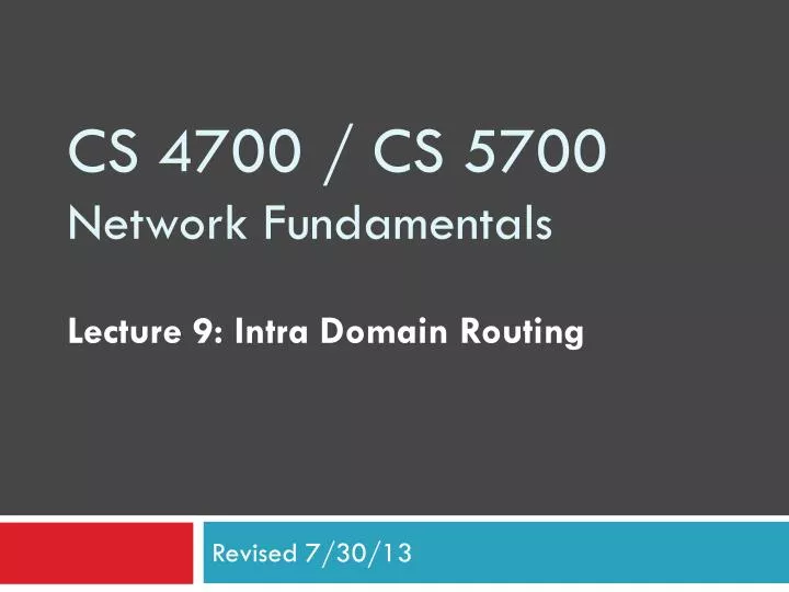
Lecture 9 : Intra Domain Routing. CS 4700 / CS 5700 Network Fundamentals. Revised 7/30/13. Network Layer, Control Plane. Function: Set up routes within a single network Key challenges: Distributing and updating routes Convergence time Avoiding loops. Data Plane. Application.

E N D
Lecture 9: Intra Domain Routing CS 4700 / CS 5700Network Fundamentals Revised 7/30/13
Network Layer, Control Plane • Function: • Set up routes within a single network • Key challenges: • Distributing and updating routes • Convergence time • Avoiding loops Data Plane Application Presentation Session Transport Network OSPF RIP BGP Control Plane Data Link Physical
Internet Routing • Internet organized as a two level hierarchy • First level – autonomous systems (AS’s) • AS – region of network under a single administrative domain • Examples: Comcast, AT&T, Verizon, Sprint, etc. • AS’s use intra-domain routing protocols internally • Distance Vector, e.g., Routing Information Protocol (RIP) • Link State, e.g., Open Shortest Path First (OSPF) • Connections between AS’s use inter-domain routing protocols • Border Gateway Routing (BGP) • De facto standard today, BGP-4
AS Example AS-1 AS-3 AS-2 Interior Routers BGP Routers
Why Do We Need ASes? Routing algorithms are not efficient enough to execute on the entire Internet topology Different organizations may use different routing policies Allows organizations to hide their internal network structure Allows organizations to choose how to route across each other (BGP) • Easier to compute routes • Greater flexibility • More autonomy/independence
Routing on a Graph • Goal: determine a “good” path through the network from source to destination • What is a good path? • Usually means the shortest path • Load balanced • Lowest $$$ cost • Network modeled as a graph • Routers nodes • Link edges • Edge cost: delay, congestion level, etc. 5 3 B C 5 2 2 1 A F 3 2 1 E D 1
Routing Problems • Assume • A network with N nodes • Each node only knows • Its immediate neighbors • The cost to reach each neighbor • How does each node learn the shortest path to every other node? 5 3 B C 5 2 2 1 A F 3 2 1 E D 1
Intra-domain Routing Protocols • Distance vector • Routing Information Protocol (RIP), based on Bellman-Ford • Routers periodically exchange reachability information with neighbors • Link state • Open Shortest Path First (OSPF), based on Dijkstra • Each network periodically floods immediate reachability information to all other routers • Per router local computation to determine full routes
Outline Distance Vector Routing RIP Link State Routing OSPF IS-IS
Distance Vector Routing • What is a distance vector? • Current best known cost to reach a destination • Idea: exchange vectors among neighbors to learn about lowest cost paths • No entry for C • Initially, only has info for immediate neighbors • Other destinations cost = ∞ • Eventually, vector is filled DV Table at Node C • Routing Information Protocol (RIP)
Distance Vector Routing Algorithm Wait for change in local link cost or message from neighbor Recomputedistance table If least cost path to any destination has changed, notify neighbors
Distance Vector Initialization Node B Node A 3 B D 2 1 1 A C 7 Initialization: for all neighbors V do ifV adjacent to A D(A, V) = c(A,V); else D(A, V) = ∞; … Node D Node C
Distance Vector: 1st Iteration Node B Node A 3 B D 2 1 1 A C 7 … loop: … else if (update D(V, Y) received from V) for all destinations Y do if (destination Y through V) D(A,Y) = D(A,V) + D(V, Y); else D(A, Y) = min(D(A, Y), D(A, V) + D(V, Y)); if(there is a new min. for dest. Y) sendD(A, Y) to all neighbors forever C C B B B B 5 2 8 4 3 3 Node D Node C D(A,C) = min(D(A,C), D(A,B)+D(B,C)) • = min(7, 2 + 1) = 3 D(A,D) = min(D(A,D), D(A,C)+D(C,D)) • = min(∞, 7 + 1) = 8 D(A,D) = min(D(A,D), D(A,B)+D(B,D)) • = min(8, 2 + 3) = 5
Distance Vector: End of 3rd Iteration Node B Node A 3 B D 2 1 1 A C 7 … loop: … else if (update D(V, Y) received from V) for all destinations Y do if (destination Y through V) D(A,Y) = D(A,V) + D(V, Y); else D(A, Y) = min(D(A, Y), D(A, V) + D(V, Y)); if(there is a new min. for dest. Y) sendD(A, Y) to all neighbors forever • Nothing changes, algorithm terminates • Until something changes… Node D Node C
loop: wait (link cost update or update message) if (c(A,V) changes by d) for all destinations Y through Vdo D(A,Y) = D(A,Y) + d else if (update D(V, Y) received from V) for all destinations Y do if (destination Y through V) D(A,Y) = D(A,V) + D(V, Y); else D(A, Y) = min(D(A, Y), D(A, V) + D(V, Y)); if (there is a new minimum for destination Y) send D(A, Y) to all neighbors forever B 4 1 A C 50 Good news travels fast 1 Node B Link Cost Changes, Algorithm Starts Algorithm Terminates Node C Time
Count to Infinity Problem B 4 1 A C 50 Bad news travels slowly 60 Node B • Node B knows D(C, A) = 5 • However, B does not know the path is C B A • Thus, D(B,A) = 6 ! Node C Time
Poisoned Reverse • If C routes through B to get to A • C tells B that D(C, A) =∞ • Thus, B won’t route to A via C B 4 1 A C 50 Does this completely solve this count to infinity problem? NO Multipath loops can still trigger the issue 60 Node B Node C Time
Outline Distance Vector Routing RIP Link State Routing OSPF IS-IS
Link State Routing Each node knows its connectivity and cost to direct neighbors Each node tells every other node this information Each node learns complete network topology Use Dijkstra to compute shortest paths
Flooding Details • Each node periodically generates Link State Packet • ID of node generating the LSP • List of direct neighbors and costs • Sequence number (64-bit, assumed to never wrap) • Time to live • Flood is reliable (ack + retransmission) • Sequence number “versions” each LSP • Receivers flood LSPs to their own neighbors • Except whoever originated the LSP • LSPs also generated when link states change
Dijkstra’s Algorithm 5 • … • Loop • find w not in S s.t.D(w) is a minimum; • add w to S; • update D(v) for all v adjacent • to w and not in S: • D(v) = min( D(v), D(w) + c(w,v) ); • until all nodes in S; Initialization: S = {A}; for all nodes v if v adjacent to A then D(v) = c(A,v); else D(v) = ∞; … 3 B C 5 2 2 1 A F 3 1 2 E D 1
OSPF vs. IS-IS • Two different implementations of link-state routing OSPF IS-IS • Favored by companies, datacenters • More optional features • Built on top of IPv4 • LSAs are sent via IPv4 • OSPFv3 needed for IPv6 • Favored by ISPs • Less “chatty” • Less network overhead • Supports more devices • Not tied to IP • Works with IPv4 or IPv6
Different Organizational Structure OSPF IS-IS • Organized around overlapping areas • Area 0 is the core network • Organized as a 2-level hierarchy • Level 2 is the backbone Area 2 Area 1 Level 1 Level 2 Level 1-2 Area 0 Area 4 Area 3
Link State vs. Distance Vector • Which is best? • In practice, it depends. • In general, link state is more popular. n = number of nodes in the graph d = degree of a given node k = number of rounds