Download
1 / 28
280 likes | 438 Views
Title. Petrophysical Analysis of Fluid Substitution in Gas Bearing Reservoirs to Define Velocity Profiles – Application of Gassmann and Krief Models. Digital Formation, Inc. November 2003. Contents. Benefits Introduction Gassmann Equation in Shaley Formation Wyllie Time Series Equation

E N D
Title Petrophysical Analysis of Fluid Substitution in Gas Bearing Reservoirs to Define Velocity Profiles – Application of Gassmann and Krief Models Digital Formation, Inc. November 2003
Contents • Benefits • Introduction • Gassmann Equation in Shaley Formation • Wyllie Time Series Equation • Linking Gassmann to Wyllie • Adding a gas term to Wyllie Equation • Krief Equation • Examples • Conclusions
Benefits – Seismic • Reliable compressional and shear curves even if no acoustic data exists. • Quantify velocity slowing due to presence of gas. • Full spectrum of fluid substitution analysis. • Reliable mechanical properties, Vp/Vs ratios. • Reliable synthetics. • Does not involve neural network or empirical correlations.
Benefits – Petrophysics • Verifies consistency of petrophysical model. • Ability to create reconstructed porosity logs using deterministic approaches.
Benefits – Engineering • Reliable mechanical property profiles for drilling and stimulation design. • Does not rely on empirical correlations, or neural network curve generation, for mechanical properties.
Introduction • A critical link between petrophysics and seismic interpretation is the influence of fluid content on acoustic and density properties. • Presented are two techniques which rigorously solve compressional and shear acoustic responses in the entire range of rock types, and assuming different fluid contents.
Gassmann Equation inShaley Formation – I • The Gassmann equation accounts for the slowing of acoustic compressional energy in the formation in the presence of gas. • There is no standard petrophysical analysis that accounts for the Gassmann response and incorporates the effect in acoustic equations (e.g. Wyllie Time-Series). • Terms in the Gassmann equation: M = Elastic modulus of the porous fluid filled rock Merf = Elastic modulus of the empty rock frame Berf = Bulk modulus of the empty rock frame Bsolid = Bulk modulus of the rock matrix and shale Bfl = Bulk modulus of the fluid in pores and in clay porosity FT = Total Porosity rB = Bulk density of the rock fluid and shale combination Vp = Compressional wave velocity
Gassmann Equation inShaley Formation – II • In shaley formation, adjustments need to be made to several of the Gassmann equation terms, including porosity and bulk modulus of the solid components. • This allows a rigorous solution to Gassmann through the full range of shaley formations. • Estimates of shear acoustic response are made using a Krief model analogy.
Wyllie Time Series Equation • In the approach presented here, we have solved the Gassmann equation in petrophysical terms, and defined a gas term for the Wyllie Time-Series equation that rigorously accounts for gas. • Original Time-Series equation: Matrix Contribution Fluid Contribution Dt = Travel time = 1/V Dtma = Travel time in matrix Dtfl = Travel time in fluid
Linking Gassmann to Wyllie • Calculate Dt values from Gassmann using fluid substitution • Liquid filled i.e. Gas saturation Sg=0 • Gas filled assuming remote (far from wellbore) gas Sg • Gas filled assuming a constant Sg of 80% • From Dt values, calculate effective fluid travel times (Dtfl) • Knowing mix of water and gas, determine effective travel time of gas (Dtgas) • Relate Dt values to gas saturation, bulk volume gas
Gassmann Sg vs. Ratio of Dtgas to Dtwet Color coding refers to porosity bins
Gassmann Bulk Volume Gas vs. Ratio Dtgas to Dtwet Color coding refers to porosity bins
Gassmann Bulk Volume Gas vs. Dtgas C2 Hyperbola = C3 C1
Adding a Gas Term to Wyllie Equation • Gas term involves C1, C2 and C3 (constants) • Equation reduces to traditional Wyllie equation when Sg=0 • If gas is present, but has not been determined from other logs, the acoustic cannot be used to determine reliable porosity values. Gas Contribution Matrix Contribution Water Contribution
Krief Equation – Part I • Krief has developed a model that is analogous to Gassmann, but also extends interpretations into the shear realm. We have similarly adapted these equations to petrophysics. Vp = Compressional wave velocity VS = Shear wave velocity rB = Bulk density of the rock fluids and matrix and shale m = Shear modulus K = Elastic modulus of the shaley porous fluid filled rock KS = Elastic modulus of the shaley formation Kf = Elastic modulus of the fluid in pores bb = Biot compressibility constant Mb = Biot coefficient FT = Total Porosity
Krief Equation – Part II • The Krief analysis gives significantly different results from Gassmann, in fast velocity systems (less change in velocity in the presence of gas as compared with Gassmann). • In slow velocity systems (high porosity, unconsolidated rocks), the two models give closely comparable results.
Examples • In all of these examples, the pseudo acoustic logs are derived from a reservoir model of porosity, matrix, clay and fluids. • There is no information from existing acoustic logs in these calculations. • On all plots, porosity scale is 0 to 40%, increasing right to left. • Slow Rocks • Gassmann DTP • Krief DTP • Krief DTP & DTS • Fast Rocks • Gassmann DTP • Krief DTP • Carbonates • Gassmann DTP • Krief DTP • Fast Rocks • Gassmann DTP & DTS • Krief DTP & DTS
Slow Rocks – Gassmann DTP Compressional shows significant slowing due to gas
Slow Rocks – Krief DTP Compressional shows significant slowing due to gas
Slow Rocks – Krief DTP & DTS Compressional shows very good comparison Ratio and Shear shows fair to good comparison
Fast Rocks – Gassmann DTP Actual compressional meanders between wet and remote Noticeable slowing due to gas
Fast Rocks – Krief DTP Actual compressional superimposes on both wet and remote Negligible slowing due to gas
Carbonates – Gassmann DTP Compressional shows slightslowing due to gas
Carbonates – Krief DTP Compressional shows negligibleslowing due to gas
Fast Rocks – Gassmann DTP/DTS Good comparison with actual Shear Ratio shows slight slowing due to gas
Fast Rocks – Krief DTP/DTS Good comparison with actual Shear Ratio shows negligible slowing due to gas
Conclusions – Part I • Pseudo acoustic logs (both compressional and shear) can be created using any combination of water, oil and gas, using either Gassmann’s or Krief’s equations for clean and the full range of shaley formations. • Comparison with actual acoustic log will show whether or not the acoustic log “sees” gas or not – gives information on invasion profile. • Pseudo acoustic logs can be created even if no source acoustic log is available. • Data from either model can be incorporated into the Wyllie Time Series equation to rigorously account for gas.
Conclusions – Part II • Interpretation yields better input to create synthetic seismograms and for rock mechanical properties. • Methodology allows for detailed comparisons among well log response, drilling information, mud logs, well test data and seismic. • In fast velocity rocks and in the presence of gas, the Krief model predicts less slowing effect than Gassmann. • In slow velocity gas-bearing rocks, both models give closely comparable results. • The techniques have been applied successfully to both clastic and carbonate reservoirs throughout North America.