Download
1 / 62
660 likes | 1.01k Views
Six Sigma - Variation. SPC - Module 1 Understanding variation and basic principles. To enable delegates to better understand variation and be able to create and analyse control charts. AIM OF SPC COURSE. OBJECTIVES. Delegates will be able to:-. Appreciate what variation is

E N D
SPC - Module 1 Understanding variation and basic principles
To enable delegates to better understand variation and be able to create and analyse control charts AIM OF SPC COURSE OBJECTIVES Delegates will be able to:- • Appreciate what variation is • Understand why it is the enemy of manufacturing • Know how we measure and calculate variation • Understand the basics of the normal distribution • Identify the two types of process variation • Understand the need for objective use of data • Produce I mR charts for variable data • Understand the basic theory behind control charts • Know how to analyse control charts
The History Of SPC • 1924 - Walter Shewhart Of Bell Telephones Develops The Control Chart Still Being Used Today • 1950 - Dr W Edwards Deming Sells SPC To Japan After World War II • 1965 - Ford Failed To Implement SPC Due To No Management Commitment • 1985 - Ford Finally Implement SPC • 1989 - Boeing roll out SPC • 1992 - BAe Decide To Implement SPC • 2002 - Airbus UK start SPC in key business areas
Variation No two products or processes are exactly alike. Variation exists because any process contains many sources of variation. The differences may be large or immeasurably small, but always present.
Variation Variation is a naturally occurring phenomenon inherent within any process. Sign your name on a piece of paper three times, even if you sign it in the same pen, straight after one another, each one will vary slightly from the last one. ------------- Signature 3 They will vary due to common cause variation. If we introduce a special cause of variation into the process, then the process will vary more than usual. ------------- Signature 1 ------------- Signature 2 ----------------- Signature 4
Rank in order of desirability Customer specification limits are the outside edge of yellow zone
Why do we need to improve our processes…. • To reduce the cost of manufacturing • Our competitors may already be leading the way • Our processes are not predictable • To improve quality By improving processes we can…. • Reduce costs • Increase revenue (sales) • Have happier customers • Make our jobs more secure • Increase job satisfaction
So what to do….? • Commit to improving quality - make process capability measurable and reportable. So we will know we are getting better. • Solve problems as a team rather than individuals. Teams get better and more permanent improvements than individual efforts. • Gain better understanding of our process by studying measurement data in an informed way (control charts) • Consider all possible pitfalls when implementing improvements. • When improvements are made - make them permanent ones.
Quality of data: We may have lots of data, but …. Does it represent the process outputs we are interested in ? Is it representative of our current process ? Can we split it into subsets to aid problem solving ? Can it be paired with process inputs ? Is the operational definition for how measurements are taken and data recorded ? Has the measurement system been assessed for stability and reliability (gauge R&R) Garbage in, garbage out !
Attribute (discrete) data is that which can be counted Examples: Broken or unbroken? On or Off? Variable (continuous) data is that which can be physically be measured on a continuous scale Examples: Temperature Weight Attribute Vs. Variable data
Attribute Vs. Variable data Which type of data ? Variable Attribute ü Length in millimeters SMC (standard manufacturing cost) Number of breakdowns per day Average daily temperature Proportion of defective items Number of spars with concession Lead time (days) Mean time between failure ü ü ü ü ü ü ü
Which is best ? Variable data should be the preferred type as it tells us more about what is happening to a process. Attribute - tells us little about the process Variable - gives plenty of insight into the process
Histogram A GRAPHICAL REPRESENTATION OF DATA SHOWING HOW THE VALUES ARE DISTRIBUTED BY: • Displaying The Distribution Of Data • Displaying Process Variability (Spread) • Identifying Data Concentration
Histogram • Graphic Representation of The Data • Bar Chart • Vertical (y) axis shows the frequency of occurrence • Horizontal (x) axis shows increasing values Note : To produce histograms quickly use Excel’s Data Analysis Tool pack. 9.1 9.2 9.3 9.4 9.5 9.6
The sample Average or Mean. • Example • A set of numbers: • 3,6,9,7,5,9,10,0,4,3 • Total = 56 • Average = 56 = 5.6 10
The Sample Range • Use The Following Dataset • 5,2,9,12,3,19,7,5 The Sample Range is the largest value minus the smallest value • 19-2=17 • The Range = 17
The Normal Distribution Curve The normal curve illustrates how most measurement data is distributed around an average value. Probability of individual values are not uniform Typical process range Examples Weight of component Wing skin thickness
Characteristics Of The Normal Curve • Single peaked • Bell shaped • Average is centred • 50% above & below the average • Extends to infinity (in theory)
How do we measure variation ? Variation in a process can be measured by calculating the ‘standard deviation’ The Formula =s= S(c -c)² n-1
The Standard Deviation • Use The Following Dataset • 5,2,9,12,3,19,7,5 • The Formula = s= S(x-x )² n-1 • (5-7.75)²+(2-7.75)²+(9-7.75)².....(5-7.75)² 7 i Note : In excel you can use the STDEV function. It’s quicker than pen & paper !
Normal Distribution Proportion 68.3% 0 -4 -3 -2 -1 1 2 3 4 2s • +/- 1 Std Dev = 68.3%
Normal Distribution Proportion 95.5% -4 -3 -2 -1 0 1 2 3 4 4s • +/- 2 Std Dev = 95.5%
Normal Distribution Proportion 99.74% -4 -3 -2 -1 0 1 2 3 4 6s • +/- 3 Std Dev = 99.74%
Control charts A control chart is a run chart with control limits plotted on it. A control chart can be used to check whether a process is predictable within a range of values Control limits are an estimation of 3 standard deviations either side of the mean. 99.74% of data should be within 3 standard deviations of the mean if no ‘special cause’ variation is present.
Different types of variation Common cause - random variation • The variation that naturally exists in your process assuming ‘nothing’ changes. This type of variation is predictable in so far as you can predict the range that your process will operate within • Difficult to reduce (advanced problem solving tools required) Special cause variation • This is the type of variation is unpredictable and is exhibited in an unstable process. Variation may not look ‘normal’. No one knows what is going to happen next ! • Easy to detect and reduce (but only if robust control systems are in place)
Examples of different types of variation Common cause - random variation • Temperature • Humidity • Standard operating methods • Measurement systems • Normal running speed Special cause variation • Sudden breakdown of equipment • Power failure • Unskilled operator • Tool breakage
Objective use of data Reacting to a single item of data without first considering the normal variation expected from a process can : ...waste time and effort correcting a problem that may be due to random variation. ...increase the process variation by tampering with it thus making the process worse Using data objectively can ensure you : ...have the facts to back up your decisions. ...can quantify any improvements you make statistically
Objective use of data… In God we trust…. ….for everything else show us the data !
14 12 10 8 6 4 2 Upper spec limit = 8. Is this process in control ?
14 12 UCL 10 8 6 4 2 LCL Yes , the process is in control but not capable.
Attribute data is that which can be counted Examples: Broken or unbroken? On or Off? Variable data is that which can be physically be measured Examples: Temperature Weight Attribute Vs. Variable data
Variable Control Chart • Establishes the values of a single component characteristic measured in physical units • Product Weight (kg) • Curing Time (hrs) • Component Length (mm)
Control Chart Individual - Moving Range Charts (Also known as X-mR or I-mR) • Assumptions : • Variable data. • Normal distribution
Establish characteristic Decide on sample frequency Decide on operation to be measured Record reading & date Record any changes to the process on chart Calculate range Plot Graphs Calculate control limits Identify and take appropriate action if process out of control
Activity Exercise • Groups of 2 or 3 people • Objective: Represent a machine that cuts bar to length • ~cut drinking straws to 30mm length (approx. 20 off) • Operation: cut drinking straws • Characteristic: Length • Sample frequency: 100% • Cut by eye, 1 straw at a time to an estimated 30mm • Measure the straws in the order that they are cut • Record the information on a chart (remember to input data and update chart as you go) • One person records, one person cuts • No communication between the operator and tester.
UCL x = Xbar + 2.66 x mRbar LCL x = Xbar - 2.66 x mRbar UCL r = 3.267 x mRbar _ mRbar = CL =
Process Control Chart (iX-mR) Dept. 019 Sampling Frequency 100% Characteristic Length Chart No two Specification Limit 30mm +/- 6mm Xbar = UCL= LCL= 44 42 40 38 36 34 32 30 28 26 24 22 mR bar = CL= 10 9 8 7 6 5 4 3 2 1 0 Date Time X 38 39 36 mR ----- 1 3 UCL x = X + 2.66 x mR bar bar LCL x = X - 2.66 x mR bar bar UCL r = 3.267 x mR bar X X X _ X X
Process Control Chart (iX-mR) Dept. 019 Sampling Frequency 100% Characteristic Length Chart No two Specification Limit 30mm +/- 6mm Xbar = UCL= LCL= 44 42 40 38 36 34 32 30 28 26 24 22 mR bar = CL= 10 9 8 7 6 5 4 3 2 1 0 Date Time X 38 39 36 mR ----- 1 3 UCL x = X + 2.66 x mR bar bar LCL x = X - 2.66 x mR bar bar UCL r = 3.267 x mR bar _
X AND mR CONTROL CHART CALCULATING CONTROL LIMITS MOVING RANGE CHART _ mR _ = ENTER mR FIGURES mR = INTO CALCULATOR _ Upper Control D X mR ucl mR 4 Limit of mR = = x _ D X mR 4 AVERAGE CHART _ X _ = ENTER X FIGURES = X INTO CALCULATOR _ _ Upper Control (E mR) X + X ucl X 2 Limit of X = _ _ = + X X + (E x mR) 2 _ _ Lower Control - lcl X mR) (E X X Limit of X = 2 = _ _ X - X - (E x mR) 2
X AND mR CONTROL CHART CALCULATING CONTROL LIMITS MOVING RANGE CHART _ mR _ = ENTER mR FIGURES 2.56 mR = INTO CALCULATOR _ Upper Control D X mR ucl mR 4 Limit of mR = = 3.267 x 2.56 8.36 _ D X mR 4 AVERAGE CHART _ X _ = ENTER X FIGURES 32.6 = X INTO CALCULATOR _ _ Upper Control (E mR) X + X ucl X 2 Limit of X = 32.6 2.66 39.4 _ _ = + X 2.56 X + (E x mR) 2 _ _ Lower Control - lcl X mR) (E X X Limit of X = 2 = _ _ 32.6 2.66 2.56 25.8 X - X - (E x mR) 2
UCL x = Xbar + 2.66 x mRbar LCL x = Xbar - 2.66 x mRbar UCL r = 3.267 x mRbar _
Analysing Control Charts Shake Down • To Convert a control chart into the form of a Histogram • Turn the control chart on its side And imagine that the points would fall into a normal distribution curve
Control Chart Analysis 16 10 15 17 12 13 20 9 11 4 5 19 • Any Point Outside Control Limits 14 6 7 1 3 2 18 8 18 16 17 20 15 14 19 • A Run of 8 Points Above or Below the mean 13 12 8 10 11 6 4 7 1 9 5 2 3 • Any Non-Random Patterns 10 11 12 7 8 9 4 5 6 1 2 3
Control Chart Analysis Is there any signs of special cause present ?
Control Chart Analysis Is there any signs of special cause present ?
Control Chart Analysis Is there any signs of special cause present ?
Control Chart Analysis Any special cause here ?
Control Chart Analysis What has changed ?