Download
1 / 24
240 likes | 244 Views
Learn how to calculate the free energy of a system in chemistry using statistical thermodynamics and computational techniques. Explore the importance of entropy in chemical systems and the use of partition functions.

E N D
Computational Chemistry and Free Energy In the first seven lectures of this course the focus has been on optimising and calculating the Energy of a system. But in Chemistry the Entropy of a system is also important Therefore we would like to calculate the Free Energy of a system To do this takes more time and effort but we are going to look at some ways of doing it
Outline and Introduction In crude terms the Entropy is a measure of how mixed up things are or how many ways there are of atoms arranging themselves or the probability of a system taking up a particular structure Therefore if we can calculate the energy of every possible configuration a system can take up we should be able to calculate the free energy of the system. Hopefully this sounds a little bit familiar ??? Hopefully it sounds a bit like Statistical Thermodynamics
Stat-Therm a Reminder Statistical Thermodynamics relates molecular properties to macro-scale thermodynamic properties. In order to do this we make use of two central quantities The Bolzmann Factor and the Partition Function The Bolzmann Factor Defines the probability that a system will take up a particular configuration . It is written mathematically as: where Pjis the probability that the system is in the quantum state j with energy Ej. This can be converted to an equality because the sum of Pj over all values of j must equal 1 (because the system must be in some state).
This gives: where and the summation is carried out over all values of j or over all possible localised states. The quantity Q is the (canonical) partition function and is related to the Helmholtz free energy A by the equation: A = -kbT lnQ So Assuming it is possible to calculate the sum over all possible configurations a system can adopt, it is possible to calculate the free energy of that system. Many of the techniques used in Computational Chemistry follow Boltzman distributions therefore the calculated configuration energies can be used to provide an estimate of the partition function Q and hence calculate the free energy.
6 5 4 3 21 1 An Example Consider the (01.2) surface of the mineral hematite (Fe2O3) There are six surface Fe3+ ions in the unit cell Image we wanted to replace any two of them with another ion say Y3+ (model segregation, pollution, new materials etc. ) There 15 possible ways of doing this. Of course some will be equivalent symmetrically! If we assume that these 15 cases represent all the ways of achieving 1/3 coverage of Y3+ we could build up the partition function and use to calculate the probability the the system will take that form at a particular temperature
Configuration 12 13 14 15 16 23 24 25 26 Segregation energy / eV -0.84 -1.05 -1.02 -1.02 -0.84 -1.02 -0.84 -1.05 -1.02 Configuration 34 35 36 45 46 56 Segregation energy / eV -0.84 -0.84 -1.02 -1.02 -1.05 -0.84 Calculating the Segregation Energy for the 15 configurations we find that there are only three degenerate configurations and they fall in the ratio 6 : 3 : 6 Considering Energy alone we may expect that the configuration equivalent to 13 would form. But is this the case when we consider entropic effects as well?
12 Eseg = -0.84 eV 14 Eseg = -1.02 eV 13 Eseg = -1.05 eV Probability of observing the configuration at #K T /K 1 300 600 900 1200 1500 0% 0% 1% 5% 9% 13% 0% 42% 54% 56% 55% 54% 100% 58% 45% 39% 36% 33% The Effect of Configuration At high temperatures we would therefore expect a disordered surface
How Useful is this Really? This is interesting but considering only fifteen points is not reasonable in many cases. When Systems are larger (for example when using Molecular Dynamics) it is not possible to search all of phase space and so we will introduce inaccuracies into our calculations. We therefore need a method of searching phase space more efficiently. Fortunately lots of people have spent lots of time coming up with tricks to do just this. We will now consider some of those used most often.
Key Points • Often in chemistry entropic effects are important Need to calculate FREE ENERGY • We can do this by calculating the energy of a system in different configurations and building up a partition function • This is only possible for trivially small systems • For real systems we need to use some mathematical tricks
Free-Energy Perturbation This technique is widely used in computational biochemistry when calculating the energy difference between to two systems or in calculating the Free-Energy change associated with a chemical reaction. It is based on the simple statistical thermodynamic equations we discussed before. The free energy of a particular state A is related to the partition function Q by the equation: A = -kbT lnQ. So if Q1 and Q2 are the partition functions for states 1 and 2 then the difference in free energies between the two states is given by:
If the total energy of the system in state i is defined as Ei(p,r). Where p and r are vectors describing the momentum and position of each particle in the system then the ratio of partition functions is related to (E2-E1) by: where P1 is the Boltzmann probability function for state 1. That is the probability that state one will adopt any particular configuration in space. This is defined as: If a large number of points are sampled the integral of a function between any two limits is equal to the average value of the same function over the same range. Therefore the equation can be rewritten in the form below. Where <....> represents the average value of the function.
So What Does this Really Mean? Well it means that if we can calculate the Energy of the system in its original state and the perturbed state at lots of points in configuration space then we can calculate the free energy change. The technique is most accurate when the free energy change is small, so we normally calculate the Free Energy change over several small perturbations. DA4 DA2 DA3 DA1 DA
Type Symbol Description Mass 1 O O Water (SPC) 16.00 2 H H Water (SPC) 1.01 3 Cl- Chloride Ion 35.45 4 X- Mystery Anion 57.68 5 Br- Bromide Ion 79.90 An Example Suppose we want to calculate the difference in hydration free energy of Bromide and Chloride 1st Define a Mystery atom which is part Cl and part Br 2nd Run a MD simulation with this Mystery ion in a box of water. 3rd Re calculate the energy of each of the configuration generated in two with the mystery ion changed to Cl- and then Br- 4th Use these results to build up the the ratio of partition functions Qx/QCl and Qx/QBr. 5th Use these to calculate the free-energy change of each step and hence the overall free energy change
Key Points • Free-Energy Perturbation allows us to calculate Energy Differences more efficiently • It is most accurate when the differences are small so the energy change is normally calculated via several pseudo states For more information see: Kollman, P (1993). Free-Energy Calculations Applications to Chemical and Biochemical Phenomena,Chemical Reviews, 93(7), 2395.
Potential of Mean Force Since MD simulations can contain many thousands of atoms, often it isn’t possible to search enough of configuration space to use free energy perturbation. In some cases the method may also be inappropriate because too much time is spent searching areas that are of little importance to the overall calculation. Ideally we would like to define the important degrees of freedom and average out the unimportant degrees of freedom in such a way that the thermodynamic properties of the system are maintained. One approach is to define superatoms by lumpingseveral atoms into one interaction unit. The interactions between the atoms on the superatom are defined by potentials of mean force
The Maths: Image we have a set of co-ordinates r we can sub divide them such that r´ are the important co-ordinates and r´´ are the unimportant ones.The potential of mean force (PMF) is defined as: However this integral is hard to solve because it is defined in multidimensional space. We can however evaluate the derivative of the PMF directly from a
Which simplifies to: So the derivative of the potential of mean force is the average force acting on the important coordinates over the course of the run.
Example of Constrained Simulation Imagine we want to calculate the free-energy of an ion as it moves away from or towards a surface. One way to do this is to run a number of MD simulations where the the ion in question is fixed at a particular height from the surface. This is an example of a constrained simulation. Because we allow the ion to move freely parallel to the surface it is still scanning its constrained area of phase space. By a PMF style approach we can again show that the free energy is given by the integral, from a reference point to the constrained height, of the force acting on the constrained particle as a function of height.
Example • Consider ions of different types approaching a mineral surface. • Run several MD simulation with ion of interest fixed at varying height above the surface. • Calculate average Force acting on the ion at each height • Integrate to get the free energy as a function of height Free Energy of Ca2+ and Mg2+ approaching the (10.4) surface of CaCO3
Key Points • PMF and constrained simulations can be more efficient because we only sample the important areas of configuration space • Instead of calculating the energy directly we calculate the force acting on the atoms and integrate with respect to displacement • Both are more accurate when more configurations are sampled
Vibrational Effects So far all the techniques we have considered have been concerned with searching configurational space. In solids additional less explicit movements can also be important. These effects are related to atoms vibrating on or about their lattice site. So in order to calculate the free energy of solid state systems we need a way of calculating these vibrational effects. Since during a MD simulation we can monitor the trajectory of each atom (providing we collect data often enough) we should be able to calculate these effects. Unfortunately the vibrations happen on a very small time scale so they will become lost in the noise if we do the analysis directly.
However, we can filter the atomic trajectories using techniques used to remove noise from electronic signals. The technique involves three steps 1) The atomic trajectory information is transformed to the frequency domain. 2) A filtering function is applied to remove unwanted frequency components. 3) The data is transformed back to the time domain. After filtering the final step is to obtain the phonon density of states g(n) from the trajectories of the atomic co-ordinates. The is done by recognising that the harmonic nature of the kinetic energy distribution implies that each degree of freedom of the characteristic motions corresponds to 1/kbT of energy.
Once we have calculate the g(n) the Thermodynamic properties (Zero-Point Energy, Free Energy, Entropy etc.) of the system using relatively straight forward integrals. Density of States of Fe2O3 at 300K The accuracy of the method is dependent on the resolution of the g(n) which in turn is related to the overall length of the MD run. However since the motions are fast we also need to collect data regularly. This makes the method expensive both in cpu time and disk usage (several days of calculation and 1GB of data)
95% Confidence Interval Upper Lower Vib Surface FreeEng / Jm-2 1024 0.04 0.43 -0.35 2048 -0.31 -0.33 -0.29 4096 -0.09 -0.06 -0.11 8192 -0.07 -0.03 -0.11 Example System run using slab geometry 200ps at 300K using NVT ensemble Configurations recorded every 50 steps Density of states then calculated and the Vibrational properties Rutile - {110} Surface Ideally we would like a method for calculating the vibrational free energy directly. Fortunately a lot of research has been concerned with just that and Lattice Dynamics codes are widely available. The related theory would have been discussed in the next lecture. Instead please read the handout or look at my website.