Download
1 / 69
690 likes | 861 Views
PHYSICS I PHY 093. Zuhairusnizam Md Darus Email: znzam@salam.uitm.edu.my Phone Office : 03 5544 2140 Mobile: 012 369 0020 Website: http://zuhairusnizam.uitm.eu.my Email: znzam@salam.uitm.edu.my UiTM Shah Alam : Unit Percetakan Universiti (UPENA) UiTM Puncak Alam :Aras 4.

E N D
PHYSICS IPHY 093 Zuhairusnizam Md Darus Email: znzam@salam.uitm.edu.my Phone Office : 03 5544 2140 Mobile: 012 369 0020 Website: http://zuhairusnizam.uitm.eu.my Email: znzam@salam.uitm.edu.my UiTM Shah Alam : Unit Percetakan Universiti (UPENA) UiTM Puncak Alam :Aras 4
RECOMMENDED TEXT: PHYSICS For Scientists & Engineers With Modern Physics by Giancoli, 4th Edition REFERENCES: Fundamental of Physics by Halliday, Resnick, Walker;6th or 7th Ed., John Wiley &Sons, Inc. Physical Quantities and Units Base Quantities and SI Units Significant Figures Conversion of Units Dimensional Analysis Scalars and Vectors 1, 2 Laws of Thermodyn Heat Capacity of Gases Work and Internal Energy First Law of Thermodynamics Second Law of Thermodynamics 15 Ch 1, 3, 7 Ch 19, 20 ASSESSMENT: TESTS – 30% LAB REPORTS – 10% FINAL EXAM – 60 % Mechanics of Motion Motion with Constant Acceleration (1 – D) 3 Ch 2 Gases and Kinetic Theory Gas Laws and Absolute Temp Kinetic Theory of Gases 14 Mechanics of Motion Motion with Constant Acceleration (2 – D) 4 Ch 18 Ch 3 Newton’s Laws and Applications Circular Motion Uniform Circular Motion Centripetal and Angular Accn Centripetal Force 5 Temperature and Heat Temp and Thermal Eqm Thermometers and Temp Scale Thermal Expansion of Solids n Liquids Heat 13 093 Ch 4, 5 Ch 17 12 6 States of Matter Solid – Stress & Strain Young’s Modulus Fluids – Density and Pressure Archimedes’ Principle Bernoulli’s Principle Ch 12, 13 Work and Energy Work by a Varying Force KE n W-KE Theorem PE Conservation of Energy Ch 7, 8 11 Gravitation Newton’s Law of Gravitation Gravitational Field Strength Gravitational Potential Realtionship bet g and G Satellite Motion in Cicular Orbits Escape velocity 7 Ch 6 9 Ch 9 Ch 10, 11 Rotational Motion Rotational Dynamics Angular Momentum Momentum, Impulse and Collissions 8 10 B R E A K (18/7 – 25/7) Ch 12 ZuhairusnizamMdDarus Phoe: 0123690020 Off : 03 5544 2140 Unit Penerbitan Universiti (UPENA) http://zuhairusnizam.uitm.edu.my Email:znzam@salam.uitm.edu.my Statics Equilibrium of Particles Free-body diagram Equilibrium of Rigid Bodies Prepared by Prof Madya Ahmad Abd Hamid, May 2010
Units of Chapter 1 • The Nature of Science • Models, Theories, and Laws • Measurement and Uncertainty; Significant Figures • Units, Standards, and the SI System • Converting Units • Order of Magnitude: Rapid Estimating • Dimensions and Dimensional Analysis
1-1 The Nature of Science Observation: important first step toward scientific theory; requires imagination to tell what is important Theories: created to explain observations; will make predictions Observations will tell if the prediction is accurate, and the cycle goes on. No theory can be absolutely verified, although a theory can be proven false.
1-1 The Nature of Science • How does a new theory get accepted? • Predictions agree better with data • Explains a greater range of phenomena • Example: Aristotle believed that objects would return to a state of rest once put in motion. • Galileo realized that an object put in motion would stay in motion until some force stopped it.
1-1 The Nature of Science The principles of physics are used in many practical applications, including construction. Communication between architects and engineers is essential if disaster is to be avoided.
1-2 Models, Theories, and Laws Models are very useful during the process of understanding phenomena. A model creates mental pictures; care must be taken to understand the limits of the model and not take it too seriously. A theory is detailed and can give testable predictions. A law is a brief description of how nature behaves in a broad set of circumstances. A principle is similar to a law, but applies to a narrower range of phenomena.
1-3 Measurement and Uncertainty; Significant Figures No measurement is exact; there is always some uncertainty due to limited instrument accuracy and difficulty reading results. The photograph to the left illustrates this – it would be difficult to measure the width of this board more accurately than ± 1 mm.
1-3 Measurement and Uncertainty; Significant Figures Estimated uncertainty is written with a ± sign; for example: 8.8 ± 0.1 cm. Percent uncertainty is the ratio of the uncertainty to the measured value, multiplied by 100:
1-3 Measurement and Uncertainty; Significant Figures The number of significant figures is the number of reliably known digits in a number. It is usually possible to tell the number of significant figures by the way the number is written: 23.21 cm has four significant figures. 0.062 cm has two significant figures (the initial zeroes don’t count). 80 km is ambiguous—it could have one or two significant figures. If it has three, it should be written 80.0 km.
1-3 Measurement and Uncertainty; Significant Figures When multiplying or dividing numbers, the result has as many significant figures as the number used in the calculation with the fewest significant figures. Example: 11.3 cm x 6.8 cm = 77 cm. When adding or subtracting, the answer is no more accurate than the least accurate number used. The number of significant figures may be off by one; use the percentage uncertainty as a check.
1-3 Measurement and Uncertainty; Significant Figures Calculators will not give you the right number of significant figures; they usually give too many but sometimes give too few (especially if there are trailing zeroes after a decimal point). The top calculator shows the result of 2.0/3.0. The bottom calculator shows the result of 2.5 x 3.2.
1-3 Measurement and Uncertainty; Significant Figures Conceptual Example 1-1: Significant figures. Using a protractor, you measure an angle to be 30°. (a) How many significant figures should you quote in this measurement? (b) Use a calculator to find the cosine of the angle you measured.
1-3 Measurement and Uncertainty; Significant Figures Scientific notation is commonly used in physics; it allows the number of significant figures to be clearly shown. For example, we cannot tell how many significant figures the number 36,900 has. However, if we write 3.69 x 10⁴, we know it has three; if we write 3.690 x 10⁴, it has four. Much of physics involves approximations; these can affect the precision of a measurement also.
1-3 Measurement and Uncertainty; Significant Figures Accuracy vs. Precision Accuracy is how close a measurement comes to the true value. Precision is the repeatability of the measurement using the same instrument. It is possible to be accurate without being precise and to be precise without being accurate!
1-4 Units, Standards, and the SI System These are the standard SI prefixes for indicating powers of 10. Many are familiar; yotta, zetta, exa, hecto, deka, atto, zepto, and yocto are rarely used.
1-4 Units, Standards, and the SI System We will be working in the SI system, in which the basic units are kilograms, meters, and seconds. Quantities not in the table are derived quantities, expressed in terms of the base units. Other systems: cgs; units are centimeters, grams, and seconds. British engineering system has force instead of mass as one of its basic quantities, which are feet, pounds, and seconds.
1-5 Converting Units Unit conversions always involve a conversion factor. Example: 1 in. = 2.54 cm. Written another way: 1 = 2.54 cm/in. So if we have measured a length of 21.5 inches, and wish to convert it to centimeters, we use the conversion factor:
1-5 Converting Units Example 1-2: The 8000-m peaks. The fourteen tallest peaks in the world are referred to as “eight-thousanders,” meaning their summits are over 8000 m above sea level. What is the elevation, in feet, of an elevation of 8000 m?
1-6 Order of Magnitude: Rapid Estimating A quick way to estimate a calculated quantity is to round off all numbers to one significant figure and then calculate. Your result should at least be the right order of magnitude; this can be expressed by rounding it off to the nearest power of 10. Diagrams are also very useful in making estimations.
1-6 Order of Magnitude: Rapid Estimating Example 1-5: Volume of a lake. Estimate how much water there is in a particular lake, which is roughly circular, about 1 km across, and you guess it has an average depth of about 10 m.
1-6 Order of Magnitude: Rapid Estimating Example 1-6: Thickness of a page. Estimate the thickness of a page of your textbook. (Hint: you don’t need one of these!)
1-6 Order of Magnitude: Rapid Estimating Example 1-7: Height by triangulation. Estimate the height of the building shown by “triangulation,” with the help of a bus-stop pole and a friend. (See how useful the diagram is!)
1-6 Order of Magnitude: Rapid Estimating Example 1-8: Estimating the radius of Earth. If you have ever been on the shore of a large lake, you may have noticed that you cannot see the beaches, piers, or rocks at water level across the lake on the opposite shore. The lake seems to bulge out between you and the opposite shore—a good clue that the Earth is round. Suppose you climb a stepladder and discover that when your eyes are 10 ft (3.0 m) above the water, you can just see the rocks at water level on the opposite shore. From a map, you estimate the distance to the opposite shore as d ≈ 6.1 km. Use h = 3.0 m to estimate the radius R of the Earth.
1-7 Dimensions and Dimensional Analysis Dimensions of a quantity are the base units that make it up; they are generally written using square brackets. Example: Speed = distance/time Dimensions of speed: [L/T] Quantities that are being added or subtracted must have the same dimensions. In addition, a quantity calculated as the solution to a problem should have the correct dimensions.
1-7 Dimensions and Dimensional Analysis Dimensional analysis is the checking of dimensions of all quantities in an equation to ensure that those which are added, subtracted, or equated have the same dimensions. Example: Is this the correct equation for velocity? Check the dimensions: Wrong!
Summary of Chapter 1 • Theories are created to explain observations, and then tested based on their predictions. • A model is like an analogy; it is not intended to be a true picture, but to provide a familiar way of envisioning a quantity. • A theory is much more well developed, and can make testable predictions; a law is a theory that can be explained simply, and that is widely applicable. • Dimensional analysis is useful for checking calculations.
Summary of Chapter 1 • Measurements can never be exact; there is always some uncertainty. It is important to write them, as well as other quantities, with the correct number of significant figures. • The most common system of units in the world is the SI system. • When converting units, check dimensions to see that the conversion has been done properly. • Order-of-magnitude estimates can be very helpful.
Chapter 3 Vectors
3-1 Vectors and Scalars A vector has magnitude as well as direction. Some vector quantities: displacement, velocity, force, momentum A scalar has only a magnitude. Some scalar quantities: mass, time, temperature
3-2 Addition of Vectors—Graphical Methods For vectors in one dimension, simple addition and subtraction are all that is needed. You do need to be careful about the signs, as the figure indicates.
3-2 Addition of Vectors—Graphical Methods If the motion is in two dimensions, the situation is somewhat more complicated. Here, the actual travel paths are at right angles to one another; we can find the displacement by using the Pythagorean Theorem.
3-2 Addition of Vectors—Graphical Methods Adding the vectors in the opposite order gives the same result:
3-2 Addition of Vectors—Graphical Methods Even if the vectors are not at right angles, they can be added graphically by using the tail-to-tip method.
3-2 Addition of Vectors—Graphical Methods The parallelogram method may also be used; here again the vectors must be tail-to-tip.
3-3 Subtraction of Vectors, and Multiplication of a Vector by a Scalar In order to subtract vectors, we define the negative of a vector, which has the same magnitude but points in the opposite direction. Then we add the negative vector.
3-3 Subtraction of Vectors, and Multiplication of a Vector by a Scalar A vector can be multiplied by a scalarc; the result is a vector c that has the same direction but a magnitudecV. If c is negative, the resultant vector points in the opposite direction.
3-4 Adding Vectors by Components Any vector can be expressed as the sum of two other vectors, which are called its components. Usually the other vectors are chosen so that they are perpendicular to each other.
3-4 Adding Vectors by Components If the components are perpendicular, they can be found using trigonometric functions.
3-4 Adding Vectors by Components The components are effectively one-dimensional, so they can be added arithmetically.
3-4 Adding Vectors by Components • Adding vectors: • Draw a diagram; add the vectors graphically. • Choosex and y axes. • Resolve each vector into x and ycomponents. • Calculate each component using sines and cosines. • Add the components in each direction. • To find the length and direction of the vector, use: . and
3-4 Adding Vectors by Components Example 3-2: Mail carrier’s displacement. A rural mail carrier leaves the post office and drives 22.0 km in a northerly direction. She then drives in a direction 60.0° south of east for 47.0 km. What is her displacement from the post office?