Download
1 / 35
350 likes | 357 Views
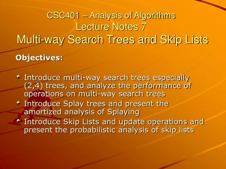
CSC401 – Analysis of Algorithms Lecture Notes 7 Multi-way Search Trees and Skip Lists. Objectives: Introduce multi-way search trees especially (2,4) trees, and analyze the performance of operations on multi-way search trees Introduce Splay trees and present the amortized analysis of Splaying

E N D
CSC401 – Analysis of Algorithms Lecture Notes 7Multi-way Search Trees and Skip Lists Objectives: • Introduce multi-way search trees especially (2,4) trees, and analyze the performance of operations on multi-way search trees • Introduce Splay trees and present the amortized analysis of Splaying • Introduce Skip Lists and update operations and present the probabilistic analysis of skip lists
A multi-way search tree is an ordered tree such that Each internal node has at least two children and stores d-1 key-element items (ki, oi), where d is the number of children For a node with children v1 v2 … vdstoring keys k1 k2 … kd-1 keys in the subtree of v1 are less than k1 keys in the subtree of vi are between ki-1 and ki(i = 2, …, d - 1) keys in the subtree of vdare greater than kd-1 The leaves store no items and serve as placeholders 11 24 2 6 8 15 27 32 30 Multi-Way Search Tree
11 24 8 12 2 6 8 15 27 32 2 4 6 14 18 10 30 1 3 5 7 9 11 13 19 16 15 17 Multi-Way Inorder Traversal • We can extend the notion of inorder traversal from binary trees to multi-way search trees • Namely, we visit item (ki, oi) of node v between the recursive traversals of the subtrees of v rooted at children vi and vi+1 • An inorder traversal of a multi-way search tree visits the keys in increasing order
11 24 2 6 8 15 27 32 30 Multi-Way Searching • Similar to search in a binary search tree • A each internal node with children v1 v2 … vd and keys k1 k2 … kd-1 • k=ki (i = 1, …, d - 1): the search terminates successfully • k<k1: we continue the search in child v1 • ki-1 <k<ki (i = 2, …, d - 1): we continue the search in child vi • k> kd-1: we continue the search in child vd • Reaching an external node terminates the search unsuccessfully • Example: search for 30
10 15 24 2 8 12 18 27 32 (2,4) Tree • A (2,4) tree (also called 2-4 tree or 2-3-4 tree) is a multi-way search with the following properties • Node-Size Property: every internal node has at most four children • Depth Property: all the external nodes have the same depth • Depending on the number of children, an internal node of a (2,4) tree is called a 2-node, 3-node or 4-node
Theorem: A (2,4) tree storing nitems has height O(log n) Proof: Let h be the height of a (2,4) tree with n items Since there are at least 2i items at depth i=0, … , h - 1 and no items at depth h, we haven1 + 2 + 4 + … + 2h-1 =2h - 1 Thus, hlog (n + 1) Searching in a (2,4) tree with n items takes O(log n) time depth items 0 1 1 2 h-1 2h-1 h 0 Height of a (2,4) Tree
We insert a new item (k, o) at the parent v of the leaf reached by searching for k We preserve the depth property but We may cause an overflow (i.e., node v may become a 5-node) Example: inserting key 30 causes an overflow 10 15 24 v 2 8 12 18 27 32 35 10 15 24 v 2 8 12 18 27 30 32 35 Insertion
Overflow and Split • We handle an overflow at a 5-node v with a split operation: • let v1 … v5 be the children of v and k1 … k4 be the keys of v • node v is replaced nodes v' and v" • v' is a 3-node with keys k1k2 and children v1v2v3 • v" is a 2-node with key k4and children v4v5 • key k3 is inserted into the parent u of v (a new root may be created) • The overflow may propagate to the parent node u u u 15 24 32 15 24 v v' v" 12 18 27 30 32 35 12 18 27 30 35 v1 v2 v3 v4 v5 v1 v2 v3 v4 v5
AlgorithminsertItem(k, o) 1. We search for key k to locate the insertion node v 2. We add the new item (k, o) at node v 3. whileoverflow(v) if isRoot(v) create a new empty root above v v split(v) Let T be a (2,4) tree with n items Tree T has O(log n) height Step 1 takes O(log n) time because we visit O(log n) nodes Step 2 takes O(1) time Step 3 takes O(log n) time because each split takes O(1) time and we perform O(log n) splits Thus, an insertion in a (2,4) tree takes O(log n) time Analysis of Insertion
10 15 24 2 8 12 18 27 32 35 10 15 27 2 8 12 18 32 35 Deletion • We reduce deletion of an item to the case where the item is at the node with leaf children • Otherwise, we replace the item with its inorder successor (or, equivalently, with its inorder predecessor) and delete the latter item • Example: to delete key 24, we replace it with 27 (inorder successor)
u u 9 14 9 w v v' 2 5 7 10 2 5 7 10 14 Underflow and Fusion • Deleting an item from a node v may cause an underflow, where node v becomes a 1-node with one child and no keys • To handle an underflow at node v with parent u, we consider two cases • Case 1: the adjacent siblings of v are 2-nodes • Fusion operation: we merge v with an adjacent sibling w and move an item from u to the merged node v' • After a fusion, the underflow may propagate to the parent u
Underflow and Transfer • To handle an underflow at node v with parent u, we consider two cases • Case 2: an adjacent sibling w of v is a 3-node or a 4-node • Transfer operation: 1. we move a child of w to v 2. we move an item from u to v 3. we move an item from w to u • After a transfer, no underflow occurs u u 4 9 4 8 w v w v 2 6 8 2 6 9
Analysis of Deletion • Let T be a (2,4) tree with n items • Tree T has O(log n) height • In a deletion operation • We visit O(log n) nodes to locate the node from which to delete the item • We handle an underflow with a series of O(log n) fusions, followed by at most one transfer • Each fusion and transfer takes O(1) time • Thus, deleting an item from a (2,4) tree takes O(log n) time
A red-black tree is a representation of a (2,4) tree by means of a binary tree whose nodes are colored red or black In comparison with its associated (2,4) tree, a red-black tree has same logarithmic time performance simpler implementation with a single node type 4 2 6 7 3 5 4 From (2,4) to Red-Black Trees 5 3 6 OR 3 5 2 7
Splay Tree Definition • a splay tree is a binary search tree where a node is splayed after it is accessed (for a search or update) • deepest internal node accessed is splayed • splaying costs O(h), where h is height of the tree – which is still O(n) worst-case • O(h) rotations, each of which is O(1) • Binary Search Tree Rules: • items stored only at internal nodes • keys stored at nodes in the left subtree of v are less than or equal to the key stored at v • keys stored at nodes in the right subtree of v are greater than or equal to the key stored at v • An inorder traversal will return the keys in order • Search proceeds down the tree to the found item or an external node.
Splay Trees do Rotations after Every Operation (Even Search) • new operation: splay • splaying moves a node to the root using rotations • right rotation • makes the left child x of a node y into y’s parent; y becomes the right child of x • left rotation • makes the right child y of a node x into x’s parent; x becomes the left child of y y x a right rotation about y a left rotation about x y T1 x T3 x y T3 T1 T2 T2 y T1 x T3 T3 T2 T1 T2 (structure of tree above x is not modified) (structure of tree above y is not modified)
Splaying: • “x is aleft-left grandchild” means x is a left child of its parent, which is itself a left child of its parent • p is x’s parent; g is p’s parent start with node x is x a left-left grandchild? is x the root? zig-zig yes stop right-rotate about g, right-rotate about p yes no is x a right-right grandchild? zig-zig is x a child of the root? no left-rotate about g, left-rotate about p yes is x a right-left grandchild? yes zig-zag is x the left child of the root? left-rotate about p, right-rotate about g no yes is x a left-right grandchild? zig zig zig-zag yes right-rotate about p, left-rotate about g right-rotate about the root left-rotate about the root yes
zig-zag x z z z y y T4 T1 y T1 T2 T3 T4 T4 x T3 x T2 T3 T1 T2 zig-zig y zig x T4 x T1 x y w T2 y z T3 w T1 T2 T3 T4 T3 T4 T1 T2 Visualizing the Splaying Cases
(20,Z) (20,Z) (10,A) (35,R) (35,R) (8,N) x g (14,J) (7,T) (10,A) (21,O) (37,P) p (21,O) (37,P) (20,Z) (10,A) g (36,L) (40,X) (1,Q) (8,N) (36,L) (40,X) (35,R) (8,N) x (14,J) (14,J) (7,T) (7,T) (1,C) (10,U) (21,O) (37,P) (5,H) p (7,P) (1,Q) (1,Q) (36,L) (40,X) (2,R) (5,G) (1,C) (1,C) (10,U) (10,U) (5,H) (5,H) (7,P) (7,P) (6,Y) (5,I) (2,R) (2,R) (5,G) (5,G) (6,Y) (6,Y) (5,I) (5,I) Splaying Example g 1. (before rotating) p • let x = (8,N) • x is the right child of its parent, which is the left child of the grandparent • left-rotate around p, then right-rotate around g x 2.(after first rotation) 3. (after second rotation) x is not yet the root, so we splay again
(20,Z) (35,R) (8,N) x (8,N) x (10,A) (21,O) (37,P) (20,Z) (36,L) (40,X) (35,R) (10,A) (21,O) (37,P) (14,J) (14,J) (7,T) (7,T) (36,L) (40,X) (1,Q) (1,Q) (1,C) (1,C) (10,U) (10,U) (5,H) (5,H) (7,P) (7,P) (2,R) (2,R) (5,G) (5,G) (6,Y) (6,Y) (5,I) (5,I) Splaying Example, Continued • now x is the left child of the root • right-rotate around root 2. (after rotation) 1. (before applying rotation) x is the root, so stop
(20,Z) (20,Z) (40,X) (10,A) (35,R) (10,A) (14,J) (37,P) (7,T) (14,J) (7,T) (21,O) (37,P) (35,R) (1,Q) (8,N) (40,X) (20,Z) (1,Q) (8,N) (36,L) (40,X) (21,O) (36,L) (1,C) (10,U) (5,H) (7,P) (10,A) (37,P) (2,R) (5,G) (1,C) (10,U) (5,H) (7,P) (14,J) (35,R) (7,T) (6,Y) (5,I) (1,Q) (8,N) (21,O) (36,L) (2,R) (5,G) (1,C) (10,U) (5,H) (7,P) (6,Y) (5,I) (2,R) (5,G) (6,Y) (5,I) Example Result before • tree might not be more balanced • e.g. splay (40,X) • before, the depth of the shallowest leaf is 3 and the deepest is 7 • after, the depth of shallowest leaf is 1 and deepest is 8 after second splay after first splay
Splay Trees & Ordered Dictionaries • which nodes are splayed after each operation? method splay node if key found, use that node if key not found, use parent of ending external node findElement insertElement use the new node containing the item inserted use the parent of the internal node that was actually removed from the tree (the parent of the node that the removed item was swapped with) removeElement
y zig x T4 x w y w T3 T1 T2 T3 T4 T1 T2 Amortized Analysis of Splay Trees • Running time of each operation is proportional to time for splaying. • Define rank(v) as the logn(v), where n(v) is the number of nodes in subtree rooted at v. • Costs: zig = $1, zig-zig = $2, zig-zag = $2. • Thus, cost for playing a node at depth d = $d. • Imagine that we store rank(v) cyber-dollars at each node v of the splay tree (just for the sake of analysis). • Cost per Zig -- Doing a zig at x costs at most rank’(x) - rank(x): • cost = rank’(x) + rank’(y) - rank(y) -rank(x) < rank’(x) - rank(x).
zig-zag x z z zig-zig T4 z y y T1 y T1 T2 T3 T4 T4 T3 x x T2 T3 T1 T2 x T1 y T2 z T3 T4 Cost per zig-zig and zig-zag • Doing a zig-zig or zig-zag at x costs at most 3(rank’(x) - rank(x)) - 2. • Proof: See Theorem 3.9, Page 192.
Performance of Splay Trees • Cost of splaying a node x at depth d of a tree rooted at r is at most 3(rank(r)-rank(x))-d+2 • Proof: Splaying x takes d/2 splaying substeps: • Recall: rank of a node is logarithm of its size, thus, amortized cost of any splay operation is O(log n). • In fact, the analysis goes through for any reasonable definition of rank(x). • This implies that splay trees can actually adapt to perform searches on frequently-requested items much faster than O(log n) in some cases. (See Theorems 3.10 and 3.11.)
A skip list for a set S of distinct (key, element) items is a series of lists S0, S1 , … , Sh such that Each list Si contains the special keys + and - List S0 contains the keys of S in nondecreasing order Each list is a subsequence of the previous one, i.e.,S0 S1 … Sh List Sh contains only the two special keys We show how to use a skip list to implement the dictionary ADT - + - 12 23 26 31 34 44 56 64 78 + What is a Skip List S3 S2 - 31 + S1 - 23 31 34 64 + S0
We search for a key x in a a skip list as follows: We start at the first position of the top list At the current position p, we compare x with y key(after(p)) x = y: we return element(after(p)) x > y: we “scan forward” x < y: we “drop down” If we try to drop down past the bottom list, we return NO_SUCH_KEY Example: search for 78 - + Search S3 S2 - 31 + S1 - 23 31 34 64 + S0 - 12 23 26 31 34 44 56 64 78 +
A randomized algorithm performs coin tosses (i.e., uses random bits) to control its execution It contains statements of the type b random() if b= 0 do A … else { b= 1} do B … Its running time depends on the outcomes of the coin tosses We analyze the expected running time of a randomized algorithm under the following assumptions the coins are unbiased, and the coin tosses are independent The worst-case running time of a randomized algorithm is often large but has very low probability (e.g., it occurs when all the coin tosses give “heads”) We use a randomized algorithm to insert items into a skip list Randomized Algorithms
S3 p2 - + S2 S2 - + p1 - 15 + S1 - + S1 23 p0 - 15 23 + S0 - 10 23 36 + S0 - 10 23 36 + 15 Insertion • To insert an item (x, o) into a skip list, we use a randomized algorithm: • We repeatedly toss a coin until we get tails, and we denote with i the number of times the coin came up heads • If i h, we add to the skip list new lists Sh+1, … , Si +1, each containing only the two special keys • We search for x in the skip list and find the positions p0, p1 , …, pi of the items with largest key less than x in each list S0, S1, … , Si • For j 0, …, i, we insert item (x, o) into list Sj after position pj • Example: insert key 15, with i= 2
S3 - + p2 S2 S2 - + - 34 + p1 S1 S1 - + - 23 34 + 23 p0 S0 S0 - 12 23 45 + - 12 23 45 + 34 Deletion • To remove an item with key xfrom a skip list, we proceed as follows: • We search for x in the skip list and find the positions p0, p1 , …, pi of the items with key x, where position pj is in list Sj • We remove positions p0, p1 , …, pi from the lists S0, S1, … , Si • We remove all but one list containing only the two special keys • Example: remove key 34
We can implement a skip list with quad-nodes A quad-node stores: item link to the node before link to the node after link to the node below link to the node after Also, we define special keys PLUS_INF and MINUS_INF, and we modify the key comparator to handle them x Implementation quad-node
The space used by a skip list depends on the random bits used by each invocation of the insertion algorithm We use the following two basic probabilistic facts: Fact 1: The probability of getting i consecutive heads when flipping a coin is 1/2i Fact 2: If each of n items is present in a set with probability p, the expected size of the set is np Consider a skip list with n items By Fact 1, we insert an item in list Si with probability 1/2i By Fact 2, the expected size of list Si is n/2i The expected number of nodes used by the skip list is Space Usage • Thus, the expected space usage of a skip list with n items is O(n)
The running time of the search an insertion algorithms is affected by the height h of the skip list We show that with high probability, a skip list with n items has height O(log n) We use the following additional probabilistic fact: Fact 3: If each of n events has probability p, the probability that at least one event occurs is at most np Consider a skip list with n items By Fact 1, we insert an item in list Si with probability 1/2i By Fact 3, the probability that list Si has at least one item is at most n/2i By picking i= 3log n, we have that the probability that S3log n has at least one item isat mostn/23log n= n/n3= 1/n2 Thus a skip list with n items has height at most 3log n with probability at least 1 - 1/n2 Height
The search time in a skip list is proportional to the number of drop-down steps, plus the number of scan-forward steps The drop-down steps are bounded by the height of the skip list and thus are O(log n) with high probability To analyze the scan-forward steps, we use yet another probabilistic fact: Fact 4: The expected number of coin tosses required in order to get tails is 2 When we scan forward in a list, the destination key does not belong to a higher list A scan-forward step is associated with a former coin toss that gave tails By Fact 4, in each list the expected number of scan-forward steps is 2 Thus, the expected number of scan-forward steps is O(log n) We conclude that a search in a skip list takes O(log n) expected time The analysis of insertion and deletion gives similar results Search and Update Times
A skip list is a data structure for dictionaries that uses a randomized insertion algorithm In a skip list with n items The expected space used is O(n) The expected search, insertion and deletion time is O(log n) Using a more complex probabilistic analysis, one can show that these performance bounds also hold with high probability Skip lists are fast and simple to implement in practice Summary