Download
1 / 14
240 likes | 708 Views
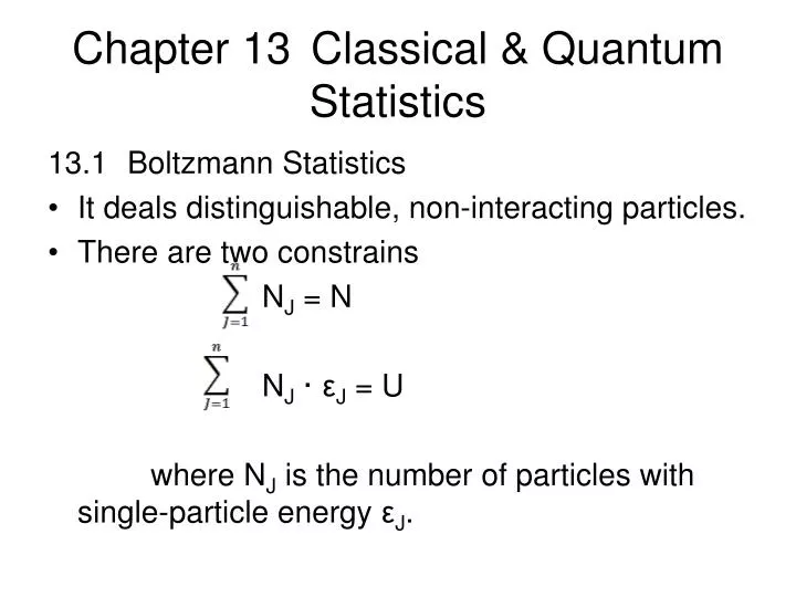
Chapter 13 Classical & Quantum Statistics. 13.1 Boltzmann Statistics It deals distinguishable, non-interacting particles. There are two constrains N J = N N J · ε J = U where N J is the number of particles with single-particle energy ε J.

E N D
Chapter 13 Classical & Quantum Statistics 13.1 Boltzmann Statistics • It deals distinguishable, non-interacting particles. • There are two constrains NJ = N NJ· εJ = U where NJ is the number of particles with single-particle energy εJ.
The goal: find the occupation number of each energy level when the thermodynamic probability is a maximum (i.e. the configuration of an equilibrium state)! • The number of ways of selecting NJ particles from a total of N to be placed in the j level is • For level 1: • For level 2, there are only (N-N1) particles left, thus
We consider that each energy level may contain more then one quantum state (degeneracy, g ≥1 )! • Using gj to represent the number of quantum state on energy level j. • Therefore, there are g1 quantum state on level 1, where each of the N1 particles would have g1 choices. Therefore, the total possibility would be g1N1. After considering the arrangement of these N1 particles W1 becomes For the second energy level, W2 becomes
The thermodynamic probability for a system with n energy levels is The above equation is subjected to two constraints listed at the beginning of this section
13.2 Lagrange multiplier • Suppose that there are only two energy levels in a system, the thermodynamic probability, W, can be expressed based on the number of particles on each level W = W (N1, N2) • The arrangement of N1 and N2, which gives the largest value of W can be found via differentiating the above equation against N1 and N2, respectively. at the maximum dw = 0
If N1 and N2 are independent variables, one has and However, N1 and N2 are connected through N = N1 + N2 For N = N(N1, N2), one has
Thus, one gets = Let the ratio be a constant = α Therefore, – α = 0 • For a system with n energy levels, there will be n differential equations. • Note that when taking the derivative against N1 , N2 , N3 ,… Nn are kept constant!
When there are two constrains, two parameters are needed! For example: N = NJ U = NJ· EJ therefore – α – β = 0 • α and β are the Lagrange multipliers.
13.3 Boltzmann Distribution Since ln W is a monotonically increasing function of W, maximizing ln W is equivalent to maximizing W. Obviously, the logarithm is much easy to work with! W = N! ) ln W = lnN! + ln( ) --- using ln (x/y) = lnx + lny ln W = lnN! + ln · gJNJ – ln NJ! --- using ln (x/y) = lnx – lny ln W =lnN! + ln ·gJNJ – ln(NJ!)--- using, again, ln (x/y) = lnx - lny Using stirlings application to the last term… ln W =lnN! + (NJlngJ) – ( NJlnNJ – NJ)
Using the method of Lagrange multiplier +α + β· = 0 Therefore, lngJ – lnNJ + α + βEJ = 0 (see chalkboard) ln = 0 + α + βEJ = eα + βEJ
The ratio of NJ/gJ is called the Boltzmann distribution, which indicates the number of particles per quantum state. Now we relate α and β to some physical properties! Since lngJ – lnNJ + α + βEJ = 0, NJ·lngJ – NJ·lnNJ + αNJ + βNJεJ = 0
Sum the above eqn over all energy levels NJ·lngJ – NJ·lnNJ + αNJ + βNJεJ = 0 NJ·lngJ – NJ·lnNJ + α·N + β·U = 0 The first two term can be replaced by lnW – lnN! –N + α·N + β·U = 0 (see in-class derivation) lnW = lnN! + N - α·N - β·U
Since S = k·lnW S = k(lnN + N - αN – βU) s = klnN - αkN -βkU But klnN + αkN = so Therefore, s = so - βkU Because T·ds = dU + P·dV = ds = + ·dV = ·dU +… therefore, =
Since s = so + k βU, = -kβ thus, = -k·β -β = = e-α·e e-α = ·e NJ = gJ e-α· e NJ = gJ·e-α· e e-α= = ·e is called partition function!