Download
1 / 99
1k likes | 1.15k Views
XPath Query Processing DBPL9 Tutorial, Sept. 8, 2003, Part 2. Georg Gottlob, TU Wien Christoph Koch, U. Edinburgh. Based on joint work with R. Pichler . Contents. Part 1 Xpath Basics Axis Evaluation Experiments with current systems Polynomial-time evaluation of Core Xpath

E N D
XPath Query ProcessingDBPL9 Tutorial, Sept. 8, 2003, Part 2 Georg Gottlob, TU Wien Christoph Koch, U. Edinburgh Based on joint work with R. Pichler
Contents Part 1 • Xpath Basics • Axis Evaluation • Experiments with current systems • Polynomial-time evaluation of Core Xpath • Core XPath and datalog • Polynomial-time evaluation of full Xpath Part 2 • Context simplification and efficient evaluation of Xpath • Parallel complexity of Xpath • Automata-based techniques: • Xpath on Streaming XML • Expressive queries and automata. • Further relevant work
Time and space bound Bottom-up evaluation based on CVT: • Time O(|data|5 * |query|2), space O(|data|4 * |query|2). Space bound (n … number of nodes in input document.): • Contexts are at most triples: at most n^3 contexts. • Sizes of values: • Node sets: at most O(n) • Strings, numbers: at most O( |data|* |query|) – (iterated concatenation of strings, multiplication of numbers) • Each CVT is of size (|data|4 * |query|). Time bound: most expensive computation is O(n^2) – Relational operation “=“ on node sets (e.g. a/b//c[d//e/f/g = h/i//j])
Alternative context representation • Contexts represented as (“previous context node, “current context node”)rather than (“context node”, “position”, “size”). • Need to recompute “position” and “size” on demand. • Complexity lowered to time O(|data|4 * |query|2), space O(|data|3 * |query|2). 0:c //a/b[position() + 1 = size()] 1:a 5:a child::b … { (1,2), (1,3), (1,4), (5,6), (5,7) } child::b[position()+1=size()] … { (1,3), (5,6) } 2:b 3:b 4:b 6:b 7:b
Context Simplification Technique • Only materialize relevant context. • Core Xpath evaluation algorithm for outermost and innermost paths //a/b/c//d[…]/e[…(a/b/c)]. • Treating “position” and “size” in a loop. • Because of tree shape of query, loops never have to be nested. /child::b[ ] (cn,cp, cs) - loop descendant::a position() = count( ) (cn) Compute node set for which child::b[…] is true (cn,cp, cs) - loop child::b[ ] position() +1 = last()
Linear Space Fragment • “Wadler Fragment” [Wadler, 1999]: Core Xpath + position(), last(), and arithmetics. • Evaluation in quadratic time and linear space. • For x in [[//a]] compute contexts (y,p,n) in x.[[b]] Compute Y = { y | (y,p,n) 2 x.[[b]] and p*2=n }. • Similarly, compute Z = { z | z.[[ d[position()*3 = last()] ]] is true}. • Compute X = { x | z 2 Z, x 2 z.[[ child::c ]]-1 } – in linear time. • Result is { w | v \in X \cap Y, w \in v.[[descendant::e]] }. (cn,cp,cs) (cn,cp,cs) //a/b[position() * 2 = last() and c/d[position()*3 = last()]]//e (cn) (cn) (cn) (cn)
Summary Full XPath • Bottom-up algorithm based on CVT • Time O(|data|5 * |query|2), space O(|data|4 * |query|2). • Top-down evaluation • Time O(|data|4 * |query|2), space O(|data|3 * |query|2). • Context-reduction technique • Time O(|data|4 * |query|2), space O(|data|2 * |query|2). Wadler fragment • Time O(|data|2 * |query|2), space O(|data| * |query|). Core Xpath • Time and space O(|data| * |query|).
Parallel Complexity of XPath • Known: Xpath is in P w.r.t. combined complexity[G., K., and Pichler, VLDB 2002]. • P-hardness => unlikely that there is an efficient parallel algorithm (conjecture: P > NC) • Even quite restrictive fragments of Xpath are P-hard • Core Xpath using only child, parent, and descendant axes, no “branching” of tree patterns. • Proof by encoding circuits, somewhat involved! • But: without negation, Core Xpath is in LOGCFL (< NC2, highly parallelizable!!)
PF – Path Query Fragment • PF = Core XPath without conditions. • E.g. //a/b//c/parent::d//f/g/ancestor::a/* • Theorem: PF is NL-complete w.r.t. combined complexity (and L-reductions). • Membership: paths easy to guess and check in NL. • NL-Hardness by reduction from Graph Reachability …
Where can we go from v2 in one step? • Reachable from v2 in one step: v1, v3!
PF is NL-hard. • Reachability in precisely m steps: • Add loop at each node to graph => reachability in at most m steps. • Set m = |E|.
Further fragments with low parallel complexity Combined complexity of Core Xpath is in L if: • Only one-step axes are used (child, parent; self). • Only transitive downward axes are used (descendant, descendant-or-self, …).
Increasing the Size of the LOGCFL Fragment • “positive Wadler fragment” [Wadler, 2000]: just like positive Core XPath, but with position arithmetics in conditions. • child::a[position()+1 = last()] … get the second-last child labeled “a”. • No iteration of predicates: child::a[…][…]. • Theorem (combined complexity): the positive WF is • LOGCFL-complete; • with iterated predicates (already when iterated at most twice), it is P-complete.
Increasing the Size of the LOGCFL Fragment • pXPath: “positive”/parallel XPath. • No negation • No iterated predicates […][…] • Depth of nesting of arithmetic operations inside a predicate is bounded by some constant. • Forbidden built-in functions: count, sum, string, local-name, name, namespace-uri, string-length, normalize-space. • Forbidden: relational operations on booleans. • Theorem. pXPath is LOGCFL-complete (combined complexity). • Maximal parallelizable fragment of Xpath, unless P = NC. • Adding any of the features (1) – (5) leads to P-hardness.
Data and Query Complexity • Theorem. PF is L-complete under NC1-reductions (data complexity). • Theorem. XPath w/o multiplication, concatenation is in L w.r.t. query complexity. • Surprisingly, data complexity and query complexity are low; combined complexity is higher! XPath PF L-complete (NC1-red.) L Data complexity
FSA on Streams • Translate Xpath path query into FSA, process stream of (e.g.) SAX events. • Very good scalability, low memory consumption (stack needed) • Selective dissemination of information (SDI) / publish-subscribe(cf. Xfilter [Altinel and Franklin, VLDB 2000], Xtrie [Chan et al., ICDE 2002]). • Boolean queries. • Extensions to support branching tree patterns, condition predicates, backward axes, … • Goal is to evaluate multiple queries at once (10^4 – 10^6 queries.)
Example: $x in //a/b b (0) a a a b b a $x $x b NFA DFA
Example: //a/b b (0) a (01) a a b b a $x $x b NFA DFA
Example: //a/b b (0) a (01) (01) a a b b a $x $x b NFA DFA
Example: //a/b b (0) a (01) (01) a a b (02) b a $x $x $x b NFA DFA
Example: //a/b b (0) a (01) (01) a a b b a $x $x $x b NFA DFA
Example: //a/b b (0) a (01) a a b b a $x $x $x b NFA DFA
Example: //a/b b (0) a (01) (01) a a b b a $x $x $x b NFA DFA
Example: //a/b b (0) a (01) a a b b a $x $x $x b NFA DFA
Example: //a/b b (0) a (01) (02) a a b $x b a $x $x $x b NFA DFA
Example: //a/b b (0) a (01) (02) a a b $x (01) b a $x $x $x b NFA DFA
Example: //a/b b (0) a (01) (02) a a b $x (01) (02) b a $x $x $x b $x NFA DFA
Example: //a/b b (0) a (01) (02) a a b $x (01) b a $x $x $x b $x NFA DFA
Example: //a/b b (0) a (01) (02) a a b $x b a $x $x $x b $x NFA DFA
Example: //a/b b (0) a (01) a a b $x b a $x $x $x b $x NFA DFA
Example: //a/b b (0) a a a b $x b a $x $x $x b $x NFA DFA
Size of DFAs //a/*/*/b
Size of DFAs • Exponential in the size of Xpath statement, but • Only exponential in number of occurrences of “*”. • In case of automaton for multiple queries, exponential in number of occurrences of “//”. • Lazy evaluation of DFA • Computation of states and transitions only on demand. • Saves much time and space in practice: documents usually from quite restrictive language. [Green, Miklau, Onizuka, Suciu, ICDT 2003]
Extensions • Branching tree patterns. • Condition predicates. • Backward axes • Boolean queries (“Can tree pattern be embedded into XML document?”) • Rather than node-selecting queries.
Motivation • Scalability in databases = (all three points at the same time) • Strictly linear time. • Little main memory required (DB in secondary storage). • Little jumping around in the data, sequential scans of disk preferred (streaming). • Paged sequential reading much faster than random access. • Node-selecting queries on unranked trees (XML) • Higher expressiveness than what is possible with single pass. • Folklore: unary MSO queries can be evaluated in two passes through the tree.
The Arb Query Processor Evaluates node-selecting queries • In two sequential scans of the data. • Memory requirements: O(depth(tree)), otherwise independent of size of DB. • Highly parallelizable. • Tree Automata-based. • High expressiveness: unary Monadic Second Order Logic (MSO). • Succinct representation of automata. [Frick, Grohe, K., LICS 2003; K., VLDB 2003]
Selecting Tree Automata (STAs) • STA: Nondeterministic bottom-up tree automatawith a set of selecting states. • Select a node if it is assigned a selecting state in all (or one) accepting runs:or • Expressive power: unary MSO queries on trees. [Neven’s thesis]; [Frick, Grohe & K., LICS 2003]
Two-Phase Query Evaluation From STA • Deterministic bottom-up tree automaton • compute reachable states. • Deterministic top-down tree automaton (with selection) • Eliminate state-to-node assignments that do not lead to accepting run. • Select nodes of query result. [Frick, Grohe & K., LICS 2003]