Download
1 / 10
100 likes | 170 Views
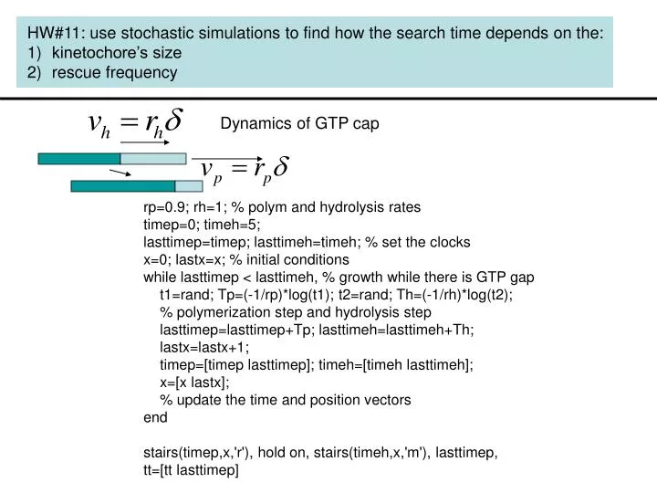
HW#11: use stochastic simulations to find how the search time depends on the: kinetochore’s size rescue frequency. Dynamics of GTP cap. rp=0.9; rh=1; % polym and hydrolysis rates timep=0; timeh=5; lasttimep=timep; lasttimeh=timeh; % set the clocks x=0; lastx=x; % initial conditions

E N D
HW#11: use stochastic simulations to find how the search time depends on the: • kinetochore’s size • rescue frequency Dynamics of GTP cap rp=0.9; rh=1; % polym and hydrolysis rates timep=0; timeh=5; lasttimep=timep; lasttimeh=timeh; % set the clocks x=0; lastx=x; % initial conditions while lasttimep < lasttimeh, % growth while there is GTP gap t1=rand; Tp=(-1/rp)*log(t1); t2=rand; Th=(-1/rh)*log(t2); % polymerization step and hydrolysis step lasttimep=lasttimep+Tp; lasttimeh=lasttimeh+Th; lastx=lastx+1; timep=[timep lasttimep]; timeh=[timeh lasttimeh]; x=[x lastx]; % update the time and position vectors end stairs(timep,x,'r'), hold on, stairs(timeh,x,'m'), lasttimep, tt=[tt lasttimep]
>> mean(tt) ans = 45.8645 >> std(tt) ans = 48.3704 >> hist(tt) Dt=5; rp=0.9; rh=1 Clear sign of exponential distribution! HW#12: use stochastic simulations to find how the catastrophe frequency depends on Does it depend on the initial conditions? Can you find appr. analytical formula and compare with stochastics? Explore both
Dt=1; rp=1.01; rh=1 z=(0:10:100);hist(tt,z) hist(tt) >> mean(tt), std(tt) ans = 235.2572 ans = 1.1192e+003
We got a problem: no reliable catastrophe at . Remember that Also, two experiments: 1) Frequency of catastrophes decreases with increasing tubulin concentration, M – easy to explain 2) In deletion experiment, catastrophe occurs independently of initial concentration – hard to explain So, random, not vectorial hydrolysis: Rate
rp=1; rh=1; h=0.3; % polym and hydrolysis rates time=0; dt=0.1; t=[time]; % set the clocks xp=5; xh=0; % initial conditions xxp=[xp]; xxh=[xh]; % set position vectors while xh < xp, % no catastrophe condition if rand<rp*dt xp=xp+1; else xp=xp; end xxp=[xxp xp]; % polymerization step if rand<h*dt xh=floor(xh+(xp-xh)*rand); elseif rand<rh*dt xh=xh+1; else xh=xh; end xxh=[xxh xh]; % hydrolysis step time=time+dt; t=[t time]; end plot(t,xxp,'r',t,xxh,'m'), time, tt=[tt time] rp=2; rh=1; h=0.3;
xp=5; rp=1; rh=1; h=0.3; >> mean(tt), std(tt) ans = 10.0400 ans = 8.8914 xp=10; rp=1; rh=1; h=0.3; >> mean(tt), std(tt) ans = 12.4340 ans = 7.5849 Independent of the initial conditions; time goes up as polym rate goes up xp=5; rp=2; rh=1; h=0.3; >> mean(tt), std(tt) ans = 44.7560 ans = 48.8262 xp=10; rp=2; rh=1; h=0.3; >> mean(tt), std(tt) ans = 37.3440 ans = 40.8963 rp=0.95; rh=1; h=0.3; 3->6, 8->12
xp=20; rp=0; rh=1; h=0.3; >> mean(tt), std(tt) ans = 8.0940 ans = 3.6961 xp=40; rp=0; rh=1; h=0.3; >> mean(tt), std(tt) ans = 11.1580 ans = 4.4341 In deletion experiment, time before catastrophe is independent of the initial conditions rp=0; rh=1; h=0.3; xp=40;
On this spatial scale, the gap is split on the same time scale it shrinks
p x