MSE 5310: Modeling Materials

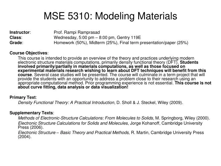
1. MSE 5310: Modeling Materials Instructor: Prof. Rampi Ramprasad Class: Wednesday, 5:00 pm – 8:00 pm, Gentry 119E Grade: Homework (50%), Midterm (25%), Final term presentation/paper (25%) Course Objectives: This course is intended to provide an overview of the theory and practices underlying modern electronic structure materials computations, primarily density functional theory (DFT). Students involved primarily/partially in materials computations, as well as those focused on experimental materials research wishing to learn about DFT techniques will benefit from this course. Several case studies will be presented. The course will culminate in a term project that will provide the students with an opportunity to address a problem close to their research using an appropriate computational method. Prior programming experience is not essential. This course is not about curve fitting, data analysis or data visualization! Primary Text: Density Functional Theory: A Practical Introduction, D. Sholl & J. Steckel, Wiley (2009). Supplementary Texts: Methods of Electronic-Structure Calculations: From Molecules to Solids, M. Springborg, Wiley (2000). Electronic Structure Calculations for Solids and Molecules, Jorge Kohanoff, Cambridge University Press (2006). Electronic Structure – Basic Theory and Practical Methods, R. Martin, Cambridge University Press (2004).

2. Planned Topics • Introduction – the course in a nutshell (Chap. 1) • Theory – From Quantum Mechanics to Density Functional Theory (Chap. 1) • Density Functional Theory (DFT) – nuts & bolts (Chap. 3) • Reciprocal space total energy formalism • Approximations – k-point sampling, pseudopotentials, exchange-correlation • Simple molecules & solids • Structure (Chap. 2) • Geometry optimization (Chap. 3) • Vibrations (Chap. 5) • Electronic structure (Chap. 8) • Surface science • Periodic boundary conditions, relaxation, reconstruction, surface energy (Chap. 4) • Chemisorption and reaction on surfaces (Chap. 4, 5, 6) • Chemical processes & transition state theory (Chap. 6) • Non-zero temperatures – Thermodynamics • Phase diagrams (Chap. 7) • Thermal properties – specific heat, thermal expansion • Response functions – elastic, dielectric, piezoelectric constants • Beyond standard DFT • Ab initio molecular dynamics (Chap. 9) • DFT + X, DFT + U, GW (Chap. 10) • Summary, outlook, accuracy of DFT (Chap. 10)

3. Lecture Topics • Introductory comments • Overview of theory: Total energy methods and density functional theory (DFT) • Predictions of known properties using DFT (i.e., validation) • Practical value of DFT calculations: Insights, and design of new materials (i.e., success stories)

4. The need for computational science • Anytime the future has to be predicted or forecasted, simulation is used, generally based on well understood scientific notions/principles • Anytime experimental analysis is too expensive or too impractical, simulation becomes necessary • Simulations complement experiments and could provide insights • Examples from everyday contemporary experience • Weather modeling involves solution of Newton’s equations of motion and fluid dynamics • Astrophysical predictions (eclipses, comets) involve solution of Newton’s equations of motion and/or general relativity • Other notable examples: economic (stock market) modeling, drug design, mechanical properties (auto industry), electromagnetic simulations (microelectronics industry) • Challenges: • Models by themselves may not be representative of the real situation • Practical treatment of model (or numerical solution) is time intensive • Sometimes the physical principles (or theory) involved are not well known • Unknown extraneous factors, e.g., stock market • Major numerical problems – non-linear systems, e,g, chaotic pendulum, weather • Fortunately, in Computational Materials Science (CMS), we need to worry mainly about the first two challenges, and the others are listed in decreasing order of importance

5. Theory, Models, Simulation & Experiments • Theory & experiment go hand in hand. • A set of results may come out of experiment, but one needs a theory to put it all in a “framework of understanding”. A theory cannot be formulated in the absence of experimental data • Goal of science: construct theory based on available experimental data, make predictions using theory outside the regime of experimental input, and modify theory if predictions are not satisfactory • A model is a representation of physical reality, along with a set of assumed equations that govern that reality • Simulation is the process of using the model using numerical techniques • CMS involves theory, modeling and simulation, with the terminologies generally used interchangeably! Theory (Understanding of Reality) Experiments (Observations of Reality) Models of Reality (in terms of atoms, electrons, etc.) Validation Simulations

6. Theory, Models, Simulation & Experiments – Example • Let us consider an example: tensile testing • In the elastic region, we know that there is a linear relationship between stress and strain, which is at the heart of elasticity theory; merely having experimental data on stress versus strain for a few materials does not constitute true understanding; the experimental data together with the realization that stress = constant*strain constitutes understanding • Now, one can do two types of computations: (1) use the constant obtained from experimental data to look at complicated geometries (FEM, used widely in the auto industry), or (2) we can use a more fundamental theory to determine the constant from first principles; the second approach results in a even more fundamental understanding of the origin of the constant, namely, in terms of atomic level bond stretching • CMS sometimes complements experimental studies, and sometimes provides insights, and increasingly is being used to design materials

7. CMS at different “scales” Time Engineering Design Years • If more than one “box” is involved in a computation  multi-scale modeling Hours Finite element Analysis (Continuum/classical) Minutes Seconds Mesoscale Modeling (Semi-classical) Microseconds Molecular Mechanics Nanoseconds Picoseconds Quantum Mechanics Femtoseconds mm nm mm m Å Distance e.g., density functional theory (DFT)

8. Overview of CMS Course – contd. • Central themes • Our system is represented as a collection of atoms, or a collection of electrons and ions • We can determine the total potential energy of this collection of particles • Equilibrium (stable, unstable and metastable) situations correspond to features (minima, maxima, saddlepoint) in the total potential energy function • Analogous approaches in other types of computations • Electromagnetic simulations involve minimization of electromagnetic energy density • Mechanical simulations involve minimization of strain energy • Let us for a moment assume that we do have a prescription for computing the total energy of a group of atoms, given their spatial positions … • What kind of properties can we compute? And how?

9. Energy RAB Diatomic molecule, A-B • Only one degree of freedom  RAB • If we new E(RAB), then we can determine potential energy surface (PES) Curvature = mw2 m = mAmB/(mA+mB) Note: slope = -force Bond energy R0 Thus, IF E(RAB) is known, then we can trivially determine equilibrium bond length, bond energy and vibrational frequency!

10. AB + C atoms E A + BC Triatomic system, A-B-C • Consider the reaction: A-B + C  A + B-C • Two degrees of freedom in 1-dimensional A-B-C system  RAB, RBC • If we new E(RAB, RBC), then we can determine potential energy surface (PES) E Activation barrier Enthalpy Transition state (saddle point) Along dot-dashed line (“reaction coordinate”)

11. Energy V Bulk cubic material • Only one degree of freedom  lattice parameter a, or Volume V (= a3) • If we new E(V), then we can determine potential energy surface (PES) Curvature = B/V0 B = bulk modulus Note: slope = stress Cohesive energy V0 Thus, IF E(V) is known [equation of state], then we can trivially determine equilibrium lattice parameter, cohesive energy and bulk modulus!

12. Lecture Topics • Introductory comments • Overview of theory: Total energy methods and density functional theory (DFT) • Predictions of known properties using DFT (i.e., validation) • Practical value of DFT calculations: Insights, and design of new materials (i.e., success stories)

13. Prescriptions for computing energy • Until ~ 1950s, no reliable prescription was available to practically compute the energy • [breakthrough: quantum mechanics, 1920s; Wigner & Seitz, 1930s; more later] • Hence energy as a function of geometry was “parameterized” using experimental data then, and even to-date! • Lennard-Jones, Morse, etc. (physicists), embedded-atom method, etc. (materials scientists), force fields (chemists) • Referred to as empirical or semi-empirical methods (as experimental data was used entirely or partially) • Today, reliable parameter-free methods are available to compute energy, which come with a (rapidly diminishing) price tag of large computational time • Density functional theory (DFT), and higher level quantum mechanics based methods

14. Empirical approach example • Suppose that our system contains M atoms, and that atoms interact “pairwise” [summation over i and j run over the number of atoms M] • Lennard-Jones: • Morse: • By fitting A and B (Lennard-Jones), or V0, d and r0 (Morse) to experimental data so that equilibrium bulk properties are reproduced, we can in principle have a scheme to compute E • We could make the scheme more sophisticated by defining E in terms of 3- or many-atom interactions (e.g., embedded atom method) or angular (e.g., Stillinger-Weber)

15. The quantum mechanical prescription • Building blocks are N electrons and M nuclei, rather than M atoms • The N-electron, M-nuclei Schrodinger (eigenvalue) equation: The N-electron, M-nuclei wave function The total energy that we seek The N-electron, M-nuclei Hamiltonian Nuclear kinetic energy Electronic kinetic energy Nuclear-nuclear repulsion Electron-electron repulsion Electron-nuclear attraction • The problem is completely parameter-free, but formidable! Why? • Cannot be solved analytically when N+M > 3 (really?!?) • Too many variables (for a 100 atom Pt cluster, the wave function is a function of 23,000 variables!!!)

16. Formidable  Manageable! • Still parameter-free, but has a few acceptable approximations • DFT is versatile: in principle, it can be used to study any atom, molecule, liquid, or solid (metals, semiconductors, insulators, polymers, etc.), at any level of dimensionality (0-d, 1-d, 2-d and 3-d) Density Functional Theory (DFT) [W. Kohn, Chemistry Nobel Prize, 1999] 1-electron wave function (function of 3 variables!) The “average” potential seen by electron i 1-electron energy (band structure energy) Energy can be obtained from r(r), or from i and ei (i labels electrons)

17. Lecture Topics • Introductory comments • Overview of theory: Total energy methods and density functional theory (DFT) • Predictions of known properties using DFT (i.e., validation) • Practical value of DFT calculations: Insights, and design of new materials (i.e., success stories)

18. The first convincing DFT calculation[Yin and Cohen, PRB 26, 5668 (1982)] • The correct equilibrium phase (diamond cubic) is predicted • The lattice parameter of the equilibrium phase, and the pressure for the diamond cubic  beta-tin phase transition (common tangent) are also predicted to a good level of accuracy Slope is transition pressure

19. Predictions of geometry • Structural details predicted typically to within 1% of experiments for a wide variety of solids and molecules • Results from various sources [collected in Ramprasad, Shi and Tang, in Physics and Chemistry of Nanodielectrics, Dielectric Polymer Nanocomposites (Springer)]

20. Predictions of other basic properties

21. Band offsets

22. Polarization in Periodic SystemsThe Fundamental Difficulty • Textbook definition • Polarization = dipole moment per unit cell volume • … inadequate … depends on how unit cell is defined … unless we are in the “Clausius-Mossotti” limit … Dipole per unit cell well defined Each unit cell will give a different net dipole Resolution provided by Resta and King-Smith & Vanderbilt, in terms of phases of the wavefunctions (Berry’s phase)

24. Phase transformations involving solids Experiments Tin Boron Nitride Kern et al, PRB 59, 8551 (1999) Pavone et al, PRB 57, 10421 (1998)

25. Phase transformations involving melting expt. expt. DFT DFT

26. Most-cited papers in APS journals • Six out of the top eleven most-cited papers are DFT-foundational papers!

27. Lecture Topics • Introductory comments • Overview of theory: Total energy methods and density functional theory (DFT) • Predictions of known properties using DFT (i.e., validation) • Practical value of DFT calculations: Insights, and design of new materials (i.e., success stories)

28. Extreme pressures • Extreme geophysical pressures may be difficult to create in the lab, but can be simulated easily

29. Extreme pressures – contd. Liquid Solid

30. Extreme pressures – contd.

31. Thermal expansion • Can a material contract when heated?

32. Si reconstruction • When heated to high temperatures in ultra high vacuum the surface atoms of the Si (111) surface rearrange to form the 7x7 reconstructed surface

33. Bi makes Cu-Cu bonds softer (hence, brittleness NOT due to electronic effects) Grain boundary decohesion due to larger size of Bi atoms

37. High activity of transition metals in oxidation catalysis is due to the presence of surface oxides under catalytic conditions

39. What can DFT (not) do? • Systems that can be represented in terms of up to a few 100 atoms per repeating unit cell are okay • Geometric details to within 1% of experiments • Other properties to within 5% of experiments • Challenges • Investigations requiring a large number of atoms • Systems in which periodicity is absent • Band gaps and excited state energies • Non-zero and high temperatures • Highly “correlated-electron” systems

40. Lecture Topics • Introductory comments • Overview of theory: Total energy methods and density functional theory (DFT) • Predictions of known properties using DFT (i.e., validation) • Practical value of DFT calculations: Insights, and design of new materials (i.e., success stories)

41. Planned Topics • Introduction – the course in a nutshell (Chap. 1) • Theory – From Quantum Mechanics to Density Functional Theory (Chap. 1) • Density Functional Theory (DFT) – nuts & bolts (Chap. 3) • Reciprocal space total energy formalism • Approximations – k-point sampling, pseudopotentials, exchange-correlation • Simple molecules & solids • Structure (Chap. 2) • Geometry optimization (Chap. 3) • Vibrations (Chap. 5) • Electronic structure (Chap. 8) • Surface science • Periodic boundary conditions, relaxation, reconstruction, surface energy (Chap. 4) • Chemisorption and reaction on surfaces (Chap. 4, 5, 6) • Chemical processes & transition state theory (Chap. 6) • Non-zero temperatures – Thermodynamics • Phase diagrams (Chap. 7) • Thermal properties – specific heat, thermal expansion • Response functions – elastic, dielectric, piezoelectric constants • Beyond standard DFT • Ab initio molecular dynamics (Chap. 9) • DFT + X, DFT + U, GW (Chap. 10) • Summary, outlook, accuracy of DFT (Chap. 10)