Download
1 / 47
500 likes | 756 Views
Instrumental variable estimation. Amine Ouazad Ass. Professor of Economics. Problemo. OLS is plagued by the problem of omitted variables… It is not a testable assumption. (remember the exercise?)

E N D
Instrumental variable estimation Amine Ouazad Ass. Professor of Economics
Problemo • OLS is plagued by the problem of omitted variables… • It is not a testable assumption.(remember the exercise?) • An instrumental variable can circumvent the problem by providing us with an “exogenous” source of variation of the covariate. • A variable that provides us with variation almost as good as a natural experiment! … without randomization.
Randomization is nice, but… • Costly & time consuming. • Ethical issues. • Individuals/Firms may not want to participate. • Only provides us with an estimate valid for our particular dataset.
Instrumental variables • Provide “natural experiment” from the comfort of your office. • The exogeneity of the variation needs to be argued, cannot be proven statistically. • Can solve the endogeneity problem for samples that have already been collected. Observational data vs experimental data
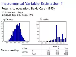
Outline • An example • Instrumental variable estimation • Implementation • The Hausman test forthe equality of OLS and IV • Instrumental variable estimationin small samples • Acemoglu, Johnson, Robinson
2. One covariate • In the regression y =a+bx+e, the covariate x is endogenous, i.e. does not satisfy A3, and Cov(e,x) is nonzero. • The variable z is an instrument if: • It predicts x: Cov(z,x) is non zero. • It is exogenous: Cov(z,e)=0. • The IV estimator is then: • = Cov(z,y)/Cov(z,x)where the cov(z,y) is the covariance in the sample. • Notice that if z = x then the IV estimator is the OLS estimator.
2 stage least squares interpretation • 2-stage least squares interpretation: • 1st stage: x = g +d z + u. • 2nd stage: y = a + b x + e. • 1st stage: regress x on z, and predict x, so that the prediction is . • 2nd stage: regress y on the prediction . • Each stage is an OLS regression. • The coefficient of in the second stage is the IV estimator of b.
Reduced form regression • The OLS regression of the dependent variable on the instrument. • y = p + j z + u. • z is exogenous. • Note that j = bd . The reduced form effect combines the first and the second stage effects.
Treatment/Control Interpretation • Assume that the interest is in looking at the causal effect of a variable x, and a treatment and control group have been set up, but the compliance of subjects is imperfect. • x = g +dD+ u . • D is a dummy for the treatment group, which affects x. • Then the IV estimator = Cov(D,y)/Cov(D,x)estimates the effect of x on y. • Notice that : • This is called the Wald estimator.
2. Multiple covariates • Consider the regression Y = Xb + e. • And we have a vector of instruments Z. • For the time being, we assume that each endogenous variable has exactly one instrument. • The exogenous variables in x are instrumented by themselves, i.e. they are in the matrix Z.
Two conditions • The instruments predict the covariates: plim (1/N) Z’X is nonzero or E(Z’X) is of full rank. • The instruments are exogenous: plim (1/N) Z’e is zeroor E(Z’e) is zero
Causal graph • Another notation for the two previous conditions. Dependent variable Instrument Y Z X Endogenous covariate e Unobservables
IV Estimator with multiple covariates • Then the IV estimator is =(Z’X)-1Z’Y. • Notice that it is equivalent to the 2SLS regression: • The prediction of the first stage regression =X(Z’Z)-1Z’X. • The regression of Y on the first stage regression = (’)-1’Y. • Exercise: Show this is equal to the IV estimator at the top of this slide.
What if the number of instruments L is different than the number of covariates K? • L < number of covariates K,model is underidentified. • L = number of covariates K,model is exactly identified. • L > number of covariates K,model is overidentified. • Why do we use these names?
2 SLS with L diff. than K • Regress X on the vector Z. • Regress Y on the predictions of X. • Notice this fails whenever L<K, because predictions will be linearly dependent (A2 fails). • But no problem if L>=K.
3. Implementation • Stata’s ivreg command: • ivreg y (x = z) w • x : endogenous variables • w : exogenous variables • z : instruments • There should be at least as many variables in z as in x. • Allows all the clustering/heteroscedasticity options as in OLS. • Standard errors correct.
Tricky Questions Can I predict x using z only? • Variables w will be used in the first stage! • They are assumed exogenous, so they are used to predict x. • Strange cases happen. • But if w is good for the second stage, w is good for the first stage. It is efficient to use the variables in w.
Two stage regression • regress x1 z w and predict x1p , xb • … • regress xK’ z w and predict xK’p, xb • for each endogenous variable • And regress y x1p … xK’p w • gives the IV estimates. • But… the standard errors are incorrect.
4. Standard errors • Standard errors in Instrumental variable regression are typically larger than in OLS. • Formula: Var()=(Z’X)-1Z’Var(e)Z(X’Z)-1. • The Sandwich formula depends on Var(e). • More interestingly… (next page)
Standard error with one covariate • The strongest the correlation between Z and X, the smaller the confidence interval. • Weakly correlated instruments give large s.e.: • The OLS standard error is inflated by the correlation between the instrument and the covariates. =
Standard errorswith multiple covariates • With multiple covariates, the instrument is strong if the F-statistic of the first stage is high. The instrument is weak otherwise. Advanced • A little issue is that the F-stat of the first-stage regression includes the exogenous covariates as well… • Hence it is possible to get a high F-stat but no significant instrument in the first stage regression. • Solution: use ivreg2 and the Angrist-Pischke F-stat (displayed in the output).
5. Hausman test • This test compares the OLS estimator and the IV estimator. • The null hypothesis is that the OLS estimator is equal to the IV estimator. • Hausman test statistic: H=()’(Var())-1() • And asymptotically, under the null hypothesis, this converges to a chi-square distribution, with number of degrees of freedom equal to the rank of the variance-covariance matrix. • In Stata: • ivreg y (x = z) w • estimates store ivresults • regress y x w • estimates store olsresults • hausmanivresultsolsresults
Right approach to the Hausman test • The Hausman test may show that your use of the IV estimator has significantly affected the point estimate of the effect of your covariate. • If you cannot reject the null, the OLS was as good as the IV strategy.
Misconceptionsabout the Hausman test • The Hausman test is sometimes called a test of “exogeneity.” But this is wrong. • Indeed, the IV estimator is valid only if the instruments are exogenous. • The OLS estimator is valid if the covariates are exogenous. • If the null is rejected, then either (i) the instruments are endogenous and the covariates are endogenous or (ii) the instruments are exogenous and the covariates are exogenous or (iii) the instruments are endogenous and the covariates are exogenous.
6. IV estimation in small samples • The IV estimator is biased. • Indeed: E(|Z,X) = b + E((Z’X)-1Z’E(e|Z,X)) • And E(e|Z,X) is nonzero ! Otherwise X would be exogenous… • So we have a problem. In finite samples, the bias of IV can be large !
Staiger and Stock (1997) • Show using simulations that the maximal bias in IV is no more than 10% of OLS we need F>10. • Maximal bias in IV is no more than 20% of that of OLS,we need F>6.5. (Advanced considerations (X Rated) • The distribution of the IV estimator is Wishart, assuming the residuals are normally distributed. • The finite sample mean of IV does not exist with a number of instruments equal to the number of covariates.)
Causal graph • Draw the causal graph using the abstract.
Graphical analysis of the first stage • Average constraint on the executive is part of the “quality of institutions.”
8. Do workers accept lower wages in exchange for health benefits? • Craig Olson, Journal of Labor Economics, 2002. • Compensating wage theory predicts that workers receiving more generous fringe benefits are paid a lower wage than comparable workers who prefer fewer fringe benefits. This study tests this prediction for employer‐provided health insurance by modeling the wages of married women employed full‐time in the labor market. Husband's union status, husband's firm size, and husband's health coverage through his job are used as instruments for his wife's own employer health insurance benefits. The estimates suggest wives with own employer health insurance accept a wage about 20% lower than what they would have received working in a job without benefits.
Causal reasoning • Write down the causal graph.
Specifications • OLS “Naïve” regression: • Problem? The effect is typically positive, which is unlikely to be causal. • First stage regression: • Alternative first stage regression:
Dataset • III. The Data and the First‐Stage Estimates • The data used in this study are from the March–June 1990–93 Current Population Surveys (CPS). The March CPSs include questions on employer‐provided health insurance and firm size. Union status and wage data are asked each month of respondents in the outgoing rotations group (ORG) subsamples. Therefore, the data were constructed by merging the March CPS with the ORG subsamples for April, May, and June for each of the 4 years. Respondents in each March survey in rotation groups 1, 2, and 3 were matched with the ORG files for, respectively, June, May, and April. March respondents in rotations groups 4 and 8 were also included because they were asked the unionization and wage questions in March. These merged March–June files were then split by gender and marital status and merged back together by household identifiers to produce a single record for each married couple. The files for the 4 years were then pooled and the analysis restricted to households where both the husband and wife were employed. The sample was then restricted to couples where the wife was employed full time (> 34 hours a week) and had an hourly wage greater than or equal to $2.00 an hour. These criteria produced a sample of 22,332 households.
Using instrumental variables • Whenever you believe there is an omitted variable bias…. • First try to assess the direction of the bias in OLS. • Then try to find an appropriate IV estimator. • Use ivreg. • Don’t forget clustering, heteroscedasticity. • Test whether the OLS is different from IV, and in what direction. Consistent with your initial interpretation? • Report first stage, reduced form, 2SLS. • Is the instrument weak? Is the sample size small? • Weak instruments, see for instance Bascle (2008)in Strategic Organization, vol 6, p285.