Download
1 / 65
660 likes | 902 Views
Real Time load balancing of parallel application. ECE696b Yeliang Zhang. Agenda. Introduction Parallel paradigms Performance analysis Real time load balancing project Other research work example Future work. What is Parallel Computing?.

E N D
Real Time load balancing of parallel application ECE696b Yeliang Zhang
Agenda • Introduction • Parallel paradigms • Performance analysis • Real time load balancing project • Other research work example • Future work
What is Parallel Computing? • Using more than one computer at the same time to solve a problem, or using a computer that has more than one processor working simultaneously (a parallel computer). • Same program can be run on different machine at the same time (SPMD) • Different program can be run on different machine at the same time (MPMD)
Why it is interesting? • Use efficiently of computer capability • Solve problems which will take single CPU machine months, or years to solve • Provide redundancy to certain application
Continue • Limits of single CPU computing • Available memory • Performance • Parallel computing allows: • Solve problems that don’t fit on a single CPU’s memory space • Solve problems that can’t be solved in a reasonable time • We can run… • Larger problems • Faster
One Application Example • Weather Modeling and Forecasting Consider 3000 X 3000 miles, and height of 11 miles. For modeling partition into segments of 0.1X0.1X0.1 cubic miles = ~1011 segments. Lets take 2-day period and parameters need to be computed every 30 min. Assume the computations take 100 instrs. A single update takes 1013 instrs. For two days we have total instrs. of 1015 . For serial computer with 1010 instrs./sec, this takes 280 hrs to predict next 48 hrs !! Lets take 1000 processors capable of 108 instrs/sec. Each processor will do 108 segments. For 2 days we have 1012 instrs. Calculation done in 3 hrs !! Currently all major weather forecast centers (US, Europe, Asia) have supercomputers with 1000s of processors.
Some Other Application • Database inquiry • Simulation super star explosion • Fluid dynamic calculation • Cosmic microwave data analysis • Ocean modeling • Genetic research
Types of Parallelism : Two Extremes • Data parallel • Each processor performs the same task on different data • Example - grid problems • Task parallel • Each processor performs a different task • Example - signal processing • Most applications fall somewhere on the continuum between these two extremes
Basics Data Parallelism • Data parallelism exploits the concurrency that derives from the application of the same operation to multiple elements of a data structure • Ex: Add 2 to all elements of an array • Ex: increase the salary of all employees with 5 years services
p1 p2 pn Typical Task Parallel Application • N tasks if not overlapped, they can be run on N processors Application Task 1 Task 2 Task n …..
Limits of Parallel Computing • Theoretical Upper Limits • Amdahl’s Law • Practical Limits • Load balancing • Non-computational sections • Other Considerations • Sometime it needs to re-write the code
Amdahl’s Law • Amdahl’s Law places a strict limit on the speedup that can be realized by using multiple processors. • Effect of multiple processors on run time • Effect of multiple processors on speed up • Where • fs = serial fraction of code • fp = parallel fraction of code • N = number of processors • tn= time to run on N processors
80 fp = 0.99 70 60 50 Amdahl's Law 40 Reality 30 20 10 Speedup 0 0 50 100 150 200 250 Number of processors Practical Limits: Amdahl’s Law vs. Reality Amdahl’s Law provides a theoretical upper limit on parallel speedup assuming that there are no costs for speedup assuming that there are no costs for communications. In reality, communications will result in afurther degradation of performance
Practical Limits: Amdahl’s Law vs. Reality • In reality, Amdahl’s Law is limited by many things: • Communications • I/O • Load balancing • Scheduling (shared processors or memory)
Other Considerations • Writing effective parallel application is difficult! • Load balance is important • Communication can limit parallel efficiency • Serial time can dominate • Is it worth your time to rewrite your application? • Do the CPU requirements justify parallelization? • Will the code be used just once?
Sources of Parallel Overhead • Interprocessor communication: Time to transfer data between processors is usually the most significant source of parallel processing overhead. • Load imbalance: In some parallel applications it is impossible to equally distribute the subtask workload to each processor. So at some point all but one processor might be done and waiting for one processor to complete. • Extra computation: Sometime the best sequential algorithm is not easily parallelizable and one is forced to use a parallel algorithm based on a poorer but easily parallelizable sequential algorithm. Sometimes repetitive work is done on each of the N processors instead of send/recv, which leads to extra computation.
Parallel program Performance Touchstone • Execution time is the principle measure of performance
Programming Parallel Computers • Programming single-processor systems is (relatively) easy due to: • single thread of execution • single address space • Programming shared memory systems can benefit from the single address space • Programming distributed memory systems is the most difficult due to multiple address spaces and need to access remote data • Both parallel systems (shared memory and distributed memory) offer ability to perform independent operations on different data (MIMD) and implement task parallelism • Both can be programmed in a data parallel, SPMD fashion
Single Program, Multiple Data (SPMD) • SPMD: dominant programming model for shared and distributed memory machines. • One source code is written • Code can have conditional execution based on which processor is executing the copy • All copies of code are started simultaneously and communicate and synch with each other periodically • MPMD: more general, and possible in hardware, but no system/programming software enables it
Shared Memory vs. Distributed Memory • Tools can be developed to make any system appear to look like a different kind of system • distributed memory systems can be programmed as if they have shared memory, and vice versa • such tools do not produce the most efficient code, but might enable portability • HOWEVER, the most natural way to program any machine is to use tools & languages that express the algorithm explicitly for the architecture.
Shared Memory Programming: OpenMP • Shared memory systems have a single address space: • applications can be developed in which loop iterations (with no dependencies) are executed by different processors • shared memory codes are mostly data parallel, ‘SPMD’ kinds of codes • OpenMP is the new standard for shared memory programming (compiler directives) • Vendors offer native compiler directives
Accessing Shared Variables • If multiple processors want to write to a shared variable at the same time there may be conflicts Processor 1 and 2 • read X • compute X+1 • write X • Programmer, language, and/or architecture must provide ways of resolving conflicts
OpenMP Example: Parallel loop !$OMP PARALLEL DO do i=1,128 b(i) = a(i) + c(i) end do !$OMP END PARALLEL DO • The first directive specifies that the loop immediately following should be executed in parallel. The second directive specifies the end of the parallel section (optional). • For codes that spend the majority of their time executing the content of simple loops, the PARALLEL DO directive can result in significant parallel performance.
MPI Basics • What is MPI? • A message-passing library specification • Extended message-passing model • Not a language or compiler specification • Not a specific implementation or product • Designed to permit the development of parallel software libraries • Designed to provide access to advanced parallel hardware for • End users • Library writers • Tool developers
Features of MPI • General • Communications combine context and group for message security • Thread safety • Point-to-point communication • Structured buffers and derived datatypes, heterogeneity. • Modes: normal(blocking and non-blocking), synchronous, ready(to allow access to fast protocol), buffered • Collective • Both built-in and user-defined collective operations. • Large number of data movement routines. • Subgroups defined directly or by topology
Performance Analysis • Performance analysis process includes: • Data collection • Data transformation • Data visualization
Data Collection Techniques • Profile • Record the amount of time spent in different parts of a program • Counters • Record either frequencies of events or cumulative times • Event Traces • Record each occurrence of various specified events
Performance Analysis Tool • Paragraph • Portable trace analysis and visualization package developed at Oak Ridge National Laboratory for MPI program • Upshot • A trace analysis and visualization package developed at Argonne National Laboratory for MPI program • SvPablo • Provides a variety of mechanisms for collecting, transforming, and visualizing data and is designed to be extensible, so that the programmer can incorporate new data formats, data collection mechanisms, data reduction modules and displays
Load Balance • Load Balance • Static load balance • The task and data distribution are determined at compile time • Not optimally because application behavior is data dependent • Dynamic load balance • Work is assigned to nodes at runtime
Load balance for heterogeneous tasks • Load balance for heterogeneous tasks is difficult • Different tasks have different costs • Data dependencies between tasks can be very complex • Consider data dependencies when doing load balancing
General load balance architecture(Research of Carnegie Mellon Univ.) • Used for dynamic load balancing and applied on heterogeneous application
General load balance architecture(continue) • Global load balancer • Includes a set of simple load balancing strategies for each of the task types • Manages the interaction between the different task types and their load balancers.
Explanation on General load balancer architecture • Task scheduler • Collects status information from the nodes and issues task migration instructions based on this information • Task scheduler supports three load balancing policies for homogeneous tasks
Why Real Time application monitoring important • A distributed and parallel application to gain high performance needs: • Acquisition and use of substantial amounts of information about programs, about the systems on which they are running, and about specific program runs. • These information is difficult to predict accurately prior to a program’s execution • Ex. Experimentation must be conducted to determine the performance effects of a program’s load on processors and communication links or of a program’s usage of certain operating system facilities
PRAGMA: An Infrastructure for Runtime Management of Grid Applications(U of A) • The overall goal of Pragma • Realize a next-generation adaptive runtime infrastructure capable of • Reactively and proactively managing and optimizing application execution • Gather current system and application state, system behavior and application performance in real time • Network control based on agent technology
Pragma addressed key challenges • Formulation of predictive performance functions • Mechanisms for application state monitoring and characterizing • Design and deployment of an active control network combining application sensors and actuators
Performance Function • Performance function hierarchically combine analytical, experimental and empirical performance models • Performance function is used along with current system/network state information to predict the application performance
Identifying Performance Function • 1. Identify the attributes that can accurately express and quantify the operation and performance of a resource • 2. Use experimental and analytical techniques to obtain the performance function • 3. Compose the component performance function to generate an overall performance function
Performance function example • Performance function model and analyze a simple network system • Two computer(PC1 and PC2) connected through an Ethernet switch • PC1 performs a matrix multiplication and sends the result to PC2 through switch • The same for PC2 • We want to find the performance function to analyze the response time(delay) for the whole application
Performance function example(continue) • Attribute • Data size • Performance function determines the application response time with respect to this attribute • Measure the task processing time in terms of data size and feed to a neural network
Performance function example(continue) Aj,bj,cj,di are constants and D is the data size
Pragma components • System characterization and abstraction component • Abstracting the current state of the underlying computational environment and predict its behavior • Application characterization component • Abstracting AMR application in terms of its communication and computational requirements
Pragma components(continue) • Active network control • Sensor • Actuator • Management/policy agents of adaptive runtime control • Policy base • A programmable database of adaptation policies used by agents and derive the overall adaptation process
Adaptive Mesh Refinement Basics • Concentrating computational effort to appropriate regions • Tracking regions in the domain that require additional resolution by overlaying finer grid over these region • Refinement proceeds recursively
System Characterization and Abstraction • Objective • Monitor, abstract and characterize the current state of the underlying computational environment • Use this information to drive the predictive performance functions and models that can estimate its performance in the near future
Agent-based runtime adaptation • The underlying mechanisms for adaptive run-time management of grid applications is realized by an active control network of sensors, actuators and management agents