Download
1 / 24
240 likes | 562 Views
Fractals. And the economy. To begin. For centuries, individuals have searched for some way, whether it be a mathematical formula or spiritual premonition, to predict the fluctuations of the global markets. As years passed, systems were created that had

E N D
Fractals And the economy
To begin... For centuries, individuals have searched for some way, whether it be a mathematical formula or spiritual premonition, to predict the fluctuations of the global markets. As years passed, systems were created that had the ability to “predict” market swings with the correct amount of study. These systems, relying on yield curves and the bell curve to gather and organize their data, had been the teachings of business teachers for decades. Then came the 1980’s…………..
Along came the Fractal During this decade of leg warmers and big hair, the study of a new form of math, known as Fractal geometry, was booming. Benoit Mandelbrot, discoverer of the famed’ Mandelbrot set, along with other mathematicians, began to investigate the inefficiencies of the current market forecasters, and the potential fractal math had in replacing these systems.
What was the problem? One may wonder, what exactly was the problem with the old systems of predicting markets. These systems, which had been in use for decades, obviously worked to some extent if they were considered valuable enough to be taught. The answer, then, can be found by examining the philosophy of the old methods and how they may be less accurate than those based on the math of fractals
The old way Many of the older methods of market prediction are based around a belief that the fluctuations of the stock market could be categorized as utter chaos. In these systems, the only way to forecast a large growth or decay is to closely observe trends and percentages on a larger picture scale to decide when to buy or sell. Such methods are so non specific, however, that the advice would be to buy a certain year as opposed to a certain week.
Chaotic or not? So, are the fluctuations of markets chaotic? This is one of the many questions addressed in Benoit Mandelbrot’s new book, The (Mis)behavior of Market, in which the fractal response is … NO!!
Why the old system is wrong. Mandelbrot and others who claim that a possible fractal system of market prediction is the best bet, heavily rely on the idea that all market fluctuations are dependent. Why do the markets fluctuate? Do brokers one day decide to panic an sell as much stock as possible, causing the markets to crash without any rhyme or reason? No, whether it is a hurricane over Cuba, destroying sugar cane crops, or the announcement of a corporate scandal, the markets fluctuate as a result of stimuli. Markets are not spontaneous.
Other Flaws There are some very basic statistics which display the gross inaccuracies found in the old systems of market forecasting. To begin, market fluctuations are believed to follow the Bell Curve as pictured below, with zero fluctuation in the center and large, outlier fluctuations at the ends. The truth behind this is that the Bell Curve is actually an extremely poor fit to the economic swings of the last century. Let’s look at some numbers…
The following chart exhibits a given minimum percentage of fluctuation for any given day, the number of such fluctuations which would occur over roughly the last century if the market followed the Bell Curve, and then finally the actually numbers of days with such fluctuation. Minimum Percentage Number for Bell Curve Actual number 3.4 percent 58 days 1,001 days 4.5 percent 6 days 366 days 1 day every 300,000 years 7 percent 48 days
Real Vs. Fake The graphs to the right were presented in Mandelbrot’s previously mentioned book on fractal applications in the economy. Two of the graphs are made from real data of economic trends, one is from a system Mandelbrot created, and another was generated by the random walk model, one of the older systems of market forecasting, used when dealing with irregular growth. The question now posed is which two are real and which are fake? Another way of exposing the defects of the old systems is through the study of real data created by both a fractal system and a non fractal based system.
Impossible! Don’t think to hard because it is virtually impossible, based on these charts, to detect which is the fake. However, by observing a different set of charts we shall be able to easily identify the fraudulent graphs.
1 down, 1 to go The graphs displayed to the right are graphs of the change in price, from moment to moment, as opposed to the initial set of graphs which only displayed the prices themselves. BUT WAIT……Which graph is the fractal model??? By observing these sets of data it becomes apparent that the 2nd model simply does not fit in. This model is indeed fake and was created by the random walk model. Unlike the other graphs which display a range of price changes, the 2nd graph is completely unique, exhibiting a steady period of similar change, failing to replicate any real data.
Here We Go The fractal model was actually number 4, however, like the initial set of graphs, it is impossible to distinguish it from the real. This graph was created by Mandelbrot with his newest model for the working of financial markets. The name of this model is Brownian motion in multifractal time; it has the simple ability to replicate the chaos known as market fluctuations. Now that we know why the old systems of the economy need to be changed, we can explore some of the fractal math which will be used in future market forecasting.
So here's the deal... It is essential that when beginning our look into the economic applications of fractals it is understood that fractals will not and can not predict the movement of individual stock prices…sorry, but you will not become rich from watching this presentation. However, there are many applications of fractals which, with the correct amount of study, can make you bundles.
The Big Deal The biggest generator of excitement surrounding this topic is the simple fact that fractals can so easily imitate the behavior of markets. As demonstrated in the earlier graphs, Mandelbrot’s system, while it is not an exact copy of an actual market fluctuation, is indistinguishable in both price and price change charts from actual market data. This is the first step.
How to form systems Mandelbrot’s latest system, Brownian motion in multifractal time, however involved it may sound, is actually somewhat simple. When generalizing different intricacies, the formation breaks down to 4 basic parts. • Draw a square and in it draw a diagonal, either representing positive or • negative linear regression.
2. Chose a generator, such as the squiggle below, in the general direction of your initial line. Iterate this line until your result is a very choppy looking Graph. Above is one such image. This graph appears chaotic yet one may see that it is an extremely predictable model of market movement …..which is why we are only half done.
Oh geeze... Step 3 is where I become a little confused, but I will try to explain as much as I can with the help of Mr. Mandelbrot to the right. 3. This part of the model creation involves the integration of a power Law. You are most likely familiar with power laws, fitting data to them in numerous applications, however the power law used in this situation is denoted by H and is derived from the square root laws of Brownian Motion. This H, which is created based on data of whatever system you may be studying, is mingled with the existing graph to alter the predictable shape.
Finished!! 4. The final step to the creation of a model is the addition of any severe vertical jumps if needed. These jumps would be added into a graph if the model failed to recognize a certain jump, but continued to follow the expected fluctuation Patterns. Below is an example of a finished model. Now just think, you can make your own fractal model of the exchange rate of the Yen!
Good News Fortunately, even if you can’t draw your own model, there is another aspect of market predicting, involving much of the same math taught in an introductory level class, which many will have the ability to do. We will now explore a method to determine how quickly a model will diverge from the actual path the real data will take.
Lya- what? Through the use of fractal math a simple equation can be used to measure the rate two neighboring graphs or trajectories diverge, with the use of the Lyapunov Exponent. Knowing how large of an impact small differences in initial conditions can make in the fractal world, it is extremely important, when attempting to replicate the behavior of a certain data set, to know how long it takes for one’s model to move a certain distance away from the real information. In the following example, the lyapunov Exponent, which is different depending on the system used, will be for the logistic function. This example is credited to J. Orlin Grabbe.
The Lyapunov exponent is expressed in the following equation: where R is the distance plus or minus around a reference trajectory E is the difference between two initial conditions e is the natural log is the Lyapunov exponent n is the step or iteration number of the point of major divergence, n is usually the variable for which we solve. EXAMPLE There are two systems modeling the fluctuation of mutual funds for the next 20 years using the logistic functions. One model has a constant path of .75 while the other starts at .7499 then moves in its orbit. Knowing that for the logistic function the Lyapunov Exponent is log 2 or .693147, at what value of n will the path of the second model leave the interval (.74,.76)
The answer is... In the problem, you know your value for R is .01, the distance + or – from the reference trajectory of .75. Also, the value of E is known, with the difference between the two initial values being .0001. This provides us with a value for all variables except n, what we are solving for. The completed equation is: Now with a little knowledge of powers, which anyone studying fractals would of course posses, the above equation can be easily solved with the answer being n= approximately 6.64. By simply rounding this number to the next largest whole number you have found the number of iterations it takes for the paths of the two trajectories to diverge out of the specific range.
Wrap up Now, with a basic knowledge of the reasons behind fractal exploration in the financial markets, as well as a slight background in the math behind these fractal applications, there is little more for anyone to do but wait. Fractals and their connections to the economy are blossoming areas of mathematical and economic study. This topic has a bright future with many brilliant minds, such as Mandelbrot, making new discoveries daily in hopes of finding order in…….. The chaos of the markets!