Download

1 / 26
260 likes | 480 Views
Formulation in wrf_to_xb and xa_to_wrf (diagnose the pressure and geopotential height). Yong-Run Guo For discussion in CWB, Taiwan 17 March 2010. WRF model and WRFVAR variables. Base State: Constant fields: Perturbation: Total – Base: Increment: 3DVAR analysis:

E N D
Formulation in wrf_to_xb and xa_to_wrf(diagnose the pressure and geopotential height) Yong-Run Guo For discussion in CWB, Taiwan 17 March 2010
WRF model and WRFVAR variables • Base State: Constant fields: • Perturbation: Total – Base: • Increment: 3DVAR analysis: • For example, pressure perturbation: grid%p • background (first guess) pressure: grid%xb%p • pressure perturbation increment: grid%xa%p • Because the base state is the constant, the total field increment is same as the perturbation increment.
FIRST GUESS WRF WRFVAR A-Grid C-Grid
Is this the hydrostatic equation? ** Here qv, qc,… are the mixing ratio. In following slides, use instead of the qv.
** here qv,… are the mixing ratio. WRF Predictive variables WRF Diagnostic variables
The full and perturbed pressure (dry + vapor), p and p’, can be computed from the base state and perturbed h, m and g (see da_transfer_wrftoxb.inc). The formulation can be found from Eq.(2.20) and (2.21) on page 9, NCAR TECHNICAL NOTE, NCAR/TN-475+STR. Why WRF did not directly use this equation to compute the total specific volume ? Here there is an approximation
The pressure is calculated from the base state and g, h, t, and min wrftoxb: ! Adapted the code from WRF module_big_step_utilities_em.F ---- ! subroutine calc_p_rho_phi Y.-R. Guo (10/20/2004) cvpm = - (1. - gas_constant/cp) cpovcv = cp / (cp - gas_constant) do k=ks,ke ! .. The base specific volume (from real.init.code):........... ppb = znu(k) * mub(i,j) + ptop ttb = (tis0 + tlp*log(ppb/ps0)) * (ps0/ppb)**kappa albn = (gas_constant/ps0) * ttb * (ppb/ps0)**cvpm ! ............................................................. qvf1 = 1. + moist(i,j,k,P_QV) / rd_over_rv aln = -1. / (mub(i,j)+mu_2(i,j)) * ( albn*mu_2(i,j) & + rdnw(k) *(ph_2(i,j,k+1) - ph_2(i,j,k)) ) ! .. total pressure: xb%p(i,j,k) = ps0 * ( (gas_constant*(ts0+t_2(i,j,k))*qvf1) / & (ps0*(aln+albn)) )**cpovcv ! .. total dry density xb%rho(i,j,k)= 1.0 / (albn+aln) ! .. pressure purtubation: p(i,j,k) = xb%p(i,j,k) - ppb enddo
Psfc for WRFVar Xb Ptop Currently in WRFVar: Is this correct? Where is the Psfc used in WRFVar? Ppert(1) Psfc, md
V X X ANALYSISWRFVAR WRF A-Grid C-Grid
Specific humidity q and water vapor mixing ratio g where psfc is the surface pressure, ptop is the model top pressure, pdsfc is the dry part of the surface pressure, and pwsfc is the wet part of the surface pressure. Differential of (1), the equation (2) is obtained for the increment . From (2), the increment can be calculated. In the WRFVar code,
So it is clear that the perturbations of m, psfc, and g are not independent. In the TC relocation, if the moist g and surface pressure psfc are modified, the m perturbation should be diagnosed. In xatowrf, md increment is computed from psfc increment and g increment: sdmd=0.0 s1md=0.0 do k=ks,ke sdmd=sdmd+q_cgrid(i,j,k)*dnw(k) s1md=s1md+(1.0+moist(i,j,k,P_QV))*dnw(k) enddo mu_cgrid(i,j)=-(xa%psfc(i,j)+xb%psac(i,j)*sdmd)/s1md
Hydrostatic assumption (Forward equation): WRF coordinate: We have Pressure perturbation equation (Tangent linear equation)
In real.init, p perturbation is computed from m and mixing ratio g, not need h and t: Perturbation of the pressure at level hkte(model top): From the levels hkte-1 to hkts ,
The pressure perturbation (not full pressure) calculated in real.exe: ! Adapted the code from "real.init.code" by Y.-R. Guo 05/13/2004: k = ke qvf1 = 0.5*(moist(i,j,k,P_QV)+moist(i,j,k,P_QV)) qvf2 = 1./(1.+qvf1) qvf1 = qvf1*qvf2 p(i,j,k) = -0.5*(mu_2(i,j)+qvf1*mub(i,j))/rdnw(k)/qvf2 do k = ke-1,1,-1 qvf1 = 0.5*(moist(i,j,k,P_QV)+moist(i,j,k+1,P_QV)) qvf2 = 1./(1.+qvf1) qvf1 = qvf1*qvf2 p(i,j,k) = p(i,j,k+1) - (mu_2(i,j)+qvf1*mub(i,j))/qvf2/rdn(k+1) enddo How to compute the pressure increment? 1, Update the , then compute the updated p perturbation. The incremnet = updated – original; 2, Develop the tangent linear code, using increments to compute the p increment.
Pressure perturbation’s Increment is calculated from the tangent linear code in xatowrf: k = ke qvf1 = 0.5*(q_cgrid(i,j,k)+q_cgrid(i,j,k)) qvf1_b = 0.5*(moist(i,j,k,P_QV)+moist(i,j,k,P_QV)) qvf2 = - qvf1 / ((1.+qvf1_b)*(1.+qvf1_b)) qvf2_b = 1./(1.+qvf1_b) qvf1 = qvf1*qvf2_b + qvf1_b*qvf2 qvf1_b = qvf1_b*qvf2_b xa%p(i,j,k) = (-0.5/rdnw(k)) * & ( (mu_cgrid(i,j)+qvf1*mub(i,j)) / qvf2_b & -(mu_2(i,j)+qvf1_b*mub(i,j))*qvf2/(qvf2_b*qvf2_b) ) do k = ke-1,1,-1 qvf1 = 0.5*(q_cgrid(i,j,k)+q_cgrid(i,j,k+1)) qvf1_b = 0.5*(moist(i,j,k,P_QV)+moist(i,j,k+1,P_QV)) qvf2 = - qvf1 / ((1.+qvf1_b)*(1.+qvf1_b)) qvf2_b = 1./(1.+qvf1_b) qvf1 = qvf1*qvf2_b + qvf1_b*qvf2 qvf1_b = qvf1_b*qvf2_b xa%p(i,j,k) = xa%p(i,j,k+1) & - (1./rdn(k+1)) * & ( (mu_cgrid(i,j)+qvf1*mub(i,j)) / qvf2_b & -(mu_2(i,j)+qvf1_b*mub(i,j))*qvf2/(qvf2_b*qvf2_b) ) enddo
When you have m, g, p and t, the full and perturbed geopotential heights, h, can be computed based on Eq. (2.9) and (2.20) on page 8 to 9, NCAR TECHNICAL NOTE, NCAR/TN-475+STR. (see da_transfer_xatowrf.inc). Note: in wrfout, there is nonhydrostatic part of geopotential height. So this part must be kept in the geopotential hieght perturbation. WRF WRFVAR: WRFVAR WRF:
Geopotetial height perturbation calculation in da_transfer_xatowrf from p, t, g, and ht, and hf: ph_full = ht(i,j) * gravity ph_xb_hd = ht(i,j) * gravity do k = ks, ke ! To obtain all of the full fields: t, p, q(mixing ratio), rho t_full = xa%t(i,j,k) + xb%t(i,j,k) p_full = xa%p(i,j,k) + xb%p(i,j,k) q_full = moist(i,j,k,P_QV) + q_cgrid(i,j,k) ! Note: According to WRF, this is the dry air density used to ! compute the geopotential height: rho_full = p_full / (gas_constant* t_full*(1.0+q_full/rd_over_rv) ) ! To compute the theta increment with the full fields: t_2(i,j,k) = t_full*(ps0/p_full)**kappa - ts0 ! The full field of analysis ph: ph_full = ph_full & - xb%dnw(k) * (xb%psac(i,j)+mu_cgrid(i,j)) / rho ! ! background hydrostatic(?) phi: ph_xb_hd = ph_xb_hd & - xb%dnw(k) * xb%psac(i,j) / xb%rho(i,j,k) ! The analysis perturbation = Hydro_ph - base_ph + nonhydro_xb_ph: ph_2(i,j,k+1) = ph_full - phb(i,j,k+1) & + (xb%hf(i,j,k+1)*gravity - ph_xb_hd) enddo Includes the nonhydrostatic height (?)
Remarks So the independent variables are m, gand t. The variables p, including the surface pressure psfc, and the geopotential height h can be diagnosed under the hydrostatic assumption. In wrfout, there is nonhydrostatic part of the geopotential height. In WRFVar (or TC relocation procedure), we can not derive the nonhydrostatic height because we did not use any prediction equations, but we can keep the original nonhydrostatic part of the geopotential height.
END THANK YOU
3DVAR + CWBNFSResults 4~5 years ago NFS2WRF & WRF2NFS
One-day Cold-start cycling run 00Z 00Z WRFVar analysis WRFVar analysis 18Z NCEP GFS 18Z NCEP GFS
圖1. NFS 45公里模式使用3DVAR資料同化技術(代號3)及最佳化客觀分析(代號O)之海棠颱風路徑預測結果比較。 24 48 72 hr op 120 193 301 km 6R 106 198 255 km
圖2. NFS 15公里模式使用3DVAR資料同化技術(代號3)及最佳化客觀分析(代號O)之 海棠颱風路徑預測結果比較 圖3. NFS15公里模式使用3DVAR資料同化技術(代號3)及最佳化客觀分析(代號O) 對05/07/16/00UTC海棠颱風路徑預測結果。 24 48 72 hr op 76 171 255 km 6R 107 149 129 km