Download
1 / 15
170 likes | 368 Views
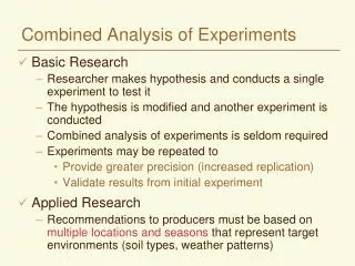
Combined Analysis of Experiments. Basic Research Researcher makes hypothesis and conducts a single experiment to test it The hypothesis is modified and another experiment is conducted Combined analysis of experiments seldom required May provide greater precision (increased replication)

E N D
Combined Analysis of Experiments • Basic Research • Researcher makes hypothesis and conducts a single experiment to test it • The hypothesis is modified and another experiment is conducted • Combined analysis of experiments seldom required • May provide greater precision (increased replication) • Validates results from initial experiment • Applied Research • Recommendations to producers must be based on multiple locations and seasons that represent target environments (soil types, weather patterns)
Multilocational trials • Often called MET = multi-environment trials • How do treatment effects change in response to differences in soil and weather throughout a region? • Detect and quantify interactions of treatments and locations and interactions of treatments and seasons in recommendation domain • Combined estimates are valid only if locations are randomly chosen within target area • Experiments often carried out on experiment stations • Generally use sites that are most accessible or convenient • Can still analyze the data, but consider possible bias due to restricted site selection when making interpretations
Preliminary Analysis • Complete ANOVA for each experiment • Did we have good data from each site? • Examine experimental errors from different locations for heterogeneity • Perform F Max test or Levene’s test for homogeneity of variance • If homogeneous, we can combine results across sites • If heterogeneous, may need to use transformation or break sites into homogeneous groups and analyze separately • Obtain preliminary estimate of interaction of treatment with environment or season • Will we be able to make general recommendations or should they be specific for each site?
Source df SS MS Expected MS Location l-1 SSL M1 Blocks in Loc. l(r-1) SSB(L) M2 Treatment t-1 SST M3 Loc. X Treatment (l-1)(t-1) SSLT M4 Pooled Error l(r-1)(t-1) SSEM5 Treatments and locations are random F for Locations = (M1+M5)/(M2+M4) Satterthwaite’s approximate df N1’ = (M1+M5)2/[(M12/(l-1))+M52/(l)(r-1)(t-1)] N2’ = (M2+M4)2/[(M22/(l-1))+M42/(l)(r-1)(t-1)] F for Treatments = M3/M4 F for Loc. x Treatments = M4/M5
Source df SS MS Expected MS Location l-1 SSL M1 Blocks in Loc. l(r-1) SSB(L) M2 Treatment t-1 SST M3 Loc. X Treatment (l-1)(t-1) SSLT M4 Pooled Error l(r-1)(t-1) SSE M5 Treatments are fixed, Locations are fixed • Fixed Locations • constitute the entire population of environments • OR • represent specific environmental conditions (rainfall, elevation, etc.) F for Locations = M1/M2 F for Treatments = M3/M5 F for Loc. x Treatments = M4/M5
Source df SS MS Expected MS Location l-1 SSL M1 Blocks in Loc. l(r-1) SSB(L) M2 Treatment t-1 SST M3 Loc. X Treatment (l-1)(t-1) SSLT M4 Pooled Error l(r-1)(t-1) SSE M5 Treatments are fixed, Locations are random F for Locations = M1/M2 F for Treatments = M3/M4 F for Loc. x Treatments = M4/M5
SAS Expected Mean Squares PROCGLM; Class Location Rep Variety; Model Yield = Location Rep(Location) Variety Location*Variety; Random Location Rep(Location) Location*Variety/Test; Source Type III Expected Mean Square Location Var(Error) + 3 Var(Location*Variety) + 7 Var(Rep(Location)) + 21 Var(Location) Dependent Variable: Yield Source DF Type III SS Mean Square F Value Pr > F Location 1 0.505125 0.505125 0.20 0.6745 Error 5.8098 15.027788 2.586644 Error: MS(Rep(Location)) + MS(Location*Variety) - MS(Error)
Source df SS MS Expected MS Years l-1 SSY M1 Blocks in Years l(r-1) SSB(Y) M2 Treatment t-1 SST M3 Years X Treatment (l-1)(t-1) SSYT M4 Pooled Error l(r-1)(t-1) SSE M5 Treatments are fixed, Years are random F for Years = M1/M2 F for Treatments = M3/M4 F for Years x Treatments = M4/M5
Locations and Years in the same trial • Can analyze as a factorial • Can determine the magnitude of the interactions between genotypes and environments (G x Y, G x L, G x Y x L) • For a simpler interpretation, can consider all year and location combinations as “sites” and use one of the models appropriate for multilocational trials
Preliminary ANOVA Assumptions for this example: - locations and blocks are random - Treatments are fixed Source df SS MS F Total lrt-1 SSTot Location l-1 SSL M1 M1/M2 Blocks in Loc. l(r-1) SSB(L) M2 Treatment t-1 SST M3 M3/M4 Loc. X Treatment (l-1)(t-1) SSLT M4 M4/M5 Pooled Error l(r-1)(t-1) SSE M5 If interactions of Loc. X Treatment are significant, must be cautious in interpreting main effects combined across all locations
Genotype by Environment Interactions (GEI) • When the relative performance of varieties differs from one location or year to another… • how do you make selections? • how do you make recommendations to farmers?
P = G + E + GE P is phenotype of an individualG is genotypeE is environment GE is the interaction 70-20-10 rule E: GE: G 20% of the observed variation among genotypes is due to interaction of genotype and environment Genotype x Environment Interactions (GEI) • How much does GEI contribute to variation among varieties or breeding lines? DeLacey et al., 1990 – summary of results from many crops and locations
Stability • Many approaches for examining GEI have been suggested since the 1960’s • Characterization of GEI is closely related to the concept of stability. “Stability” has been interpreted in different ways. • Static – performance of a genotype does not change under different environmental conditions (relevant for disease resistance, quality factors) • Dynamic – genotype performance is affected by the environment, but its relative performance is consistent across environments. It responds to environmental factors in a predictable way.
Measures of stability • CV of individual genotypes across locations • Regression of genotypes on environmental index • Eberhart and Russell, 1966 • Ecovalence • Wricke, 1962 • Superiority measure of cultivars • Lin and Binns, 1988 • Many others…
Analysis of GEI – other approaches • Rank sum index (nonparametric approach) • Cluster analysis • Factor analysis • Principal component analysis • AMMI • Pattern analysis • Analysis of crossovers • Partial Least Squares Regression • Factorial Regression