Download
1 / 23
230 likes | 336 Views
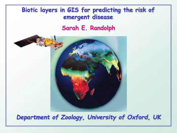
Biotic layers in GIS for predicting the risk of emergent disease. Sarah E. Randolph. Department of Zoology, University of Oxford, UK. Wildlife cycles largely hidden beneath surface. As the “iceberg” emerges, infection spills over to humans.

E N D
Biotic layers in GIS for predicting the risk of emergent disease Sarah E. Randolph Department of Zoology, University of Oxford, UK
Wildlife cycles largely hidden beneath surface • As the “iceberg” emerges, infection spills over to humans • Incidence in humans depends on bulk (transmission potential) • and relative exposure (human contact rates) of ice-berg Exposure varies in space and time Lyme borreliosis TBE (same relative exposure, smaller bulk) Commonly emergent infectious diseases arezoonoses
Two fundamental questions to answer before we can predict the risk of emergent zoonoses What determines the presence of enzootic cycles? What determines the presence of enzootic cycles? What causes the “iceberg” to grow?
Biological, process-based models • e.g. population models or transmission models • Require full quantification of rates of demographic processes Currently best available method • Statistical, pattern-matching models • Establish correlations between independent variables and observed tick presence/disease incidence • Apply and extrapolate correlations to predict risk TALA research group How to make predictive distribution maps
Disease agents Remotely sensed image Rivers Climate or Elevation Roads Vegetation or Land-use Organisms, e.g. humans or wild hosts Reality Layers in a Geographical Information System Abiotic Biotic Non-biological
Monthly NDVI for Africa Mean annual NDVI for Africa January April July October TALA research group Multi-temporal NOAA AVHRR sensor data from meteorological satellites provide seasonal images
Satellite image of land surface temperature for Europe Fourier-processed monthly data 1982-1993,mean, annual amplitude,annual phase
Disease agents Remotely sensed image Biannual phase LST Annual amplitude LST Rivers Climate or Elevation Maximum NDVI Roads Triannual amplitude NDVI Vegetation or Land-use Organisms, e.g. humans or wild hosts Reality Individual Fourier variables of satellite data as layers in a Geographical Information System
Satellite-derivedpredicteddistribution of Tick-Borne Encephalitis compared with therecorded foci(IMMUNO, 1997) across Europe Randolph SE (2000), Advances in Parasitology 47, 217-243
Two fundamental questions to answer before we can predict the risk of emergent zoonoses What determines the presence of zoonotic cycles? What causes the “iceberg” to grow? • Biotic changes? • Hosts - natural and new • Environmental changes? • Climate • Land-cover and habitats
Lyme neuroborreliosis in Denmark correlated with roe deer density temporally and spatially Annual Lyme neuroborreliosis cases Deer density per 1000ha R2 = 0.834 R2 = 0.588 R2 = 0.723 Lyme cases per county 1993-95 Tick density at 35 sites 1996 Deer density per 1000 ha Data redrawn from Jensen PM & Frandsen F (2000) Scand. J. Infect. Dis. 35, 539-44
Biotic data - major gap in GIS Disease agents Remotely sensed image Biannual phase LST Annual amplitude LST Rivers Climate or Elevation Maximum NDVI Roads Triannual amplitude NDVI Vegetation or Land-use Predicted distribution, abundance and seasonal dynamics Organisms, e.g. humans or wild hosts Reality Biological models to predict biotic data on the same scale Hosts and/or vectors
Intensive field work on small scale - many good e.gs. • Quantify the rates of demographic processes (birth & death rates) • Determine the driving forces of those rates How to make predictive biotic layers
Rhipicephalus appendiculatus Inter-stadial mortality is strongly density-dependent with significant secondary effect of moisture stress Deviations from density-dependent NN-AD mortality regression Mortality nymphs-adults R2 = 0.548 Slope = 1.360 R2 = 0.874 Mean weekly rainfall (mm) 1 month after nymphs feed Log (nymphs + 1) Randolph SE (1994) Med Vet Ent 8, 351-68
Satellite-derived NDVI correlated with mortality rates of Rhipicephalus appendiculatus ticks 2 Mean monthly mortality females to larvae 1 0.2 0.3 0.4 NDVI, 3 months after females fed
How to make predictive biotic layers • Intensive field work on small scale - many good e.gs. • Quantify the rates of demographic processes (birth & death rates) • Determine the driving forces of those rates • Biological, process-based models e.g. population models for hosts and/or vectors
Population model for the African tick Rhipicephalus appendiculatus observedandpredicted Uganda South Africa Rainfall mm/week Relative humidity Log larvae Log nymphs Log adults Month Month Randolph SE & Rogers DJ (1997) Parasitology 115, 265-79
How to make predictive biotic layers • Intensive field work on small scale - many good e.gs. • Quantify the rates of demographic processes (birth & death rates) • Determine the driving forces of those rates • Biological, process-based models e.g. population models for hosts and/or vectors • Extrapolate to large scale, driven by environmental factors in GIS
Predictive map for Rhipicephalus appendiculatus in East Africa Biological model Statistical model Observed presence
Directly transmitted diseases Enzootic cycles Wildlife host density N R0 = ____________ (h ++ r) Transmission coefficient between wildlife hosts = transmission potential Host recovery rate Host mortality rate, uninfected or infected R0 maps Spatially explicit predictions of the risk of infectious diseases • Driven by real-time changes in environmental variables
R0 maps Spatially explicit predictions of the risk of infectious diseases Directly transmitted diseases Enzootic cycles Human-wildlife contact rates and transmission coefficient Wildlife host density Human density HcN = ____________ (h ++ r) Transmission coefficient between wildlife hosts Zoonotic risk Host mortality rate, uninfected or infected • Driven by real-time changes in environmental variables • Warnings of which known zoonoses may emerge, where and when
xford Tick Research Group Past and present members of Wladimir Alonso Nick Ogden Chris Beattie Ben McCormick Noel Craine Pat Nuttall Graeme Cumming Mick Peacey Rob Green Philip Pond Andrew Hoodless Jorn Scharlemann Vicki Hughes David Strange Klaus Kurtenbach Dana Sumilo Charlie Lawrie Collaboration with:David Rogers, TALA Research group, Oxford Milan Labuda, Bratislava Lise Gern, Neuchâtel Funded by:Wellcome Trust Natural Environment Research Council, UK DEFRA EU - framework 6
TALA research group Temporal Fourier processing: seasonal characteristics of a habitat are summarized as amplitudes and phases (= timing)