Download
1 / 25
250 likes | 379 Views
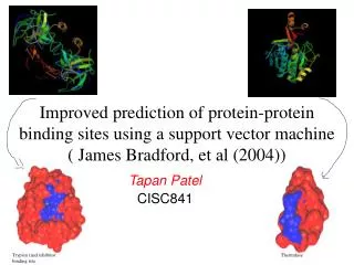
Improved prediction of protein-protein binding sites using a support vector machine ( James Bradford, et al (2004)). Tapan Patel CISC841. Trypsin (and inhibitor binding site. Thermitase. Motivation. Annotation of unknown proteins Protein structures exist whose function is not known

E N D
Improved prediction of protein-protein binding sites using a support vector machine ( James Bradford, et al (2004)) Tapan Patel CISC841 Trypsin (and inhibitor binding site Thermitase
Motivation • Annotation of unknown proteins • Protein structures exist whose function is not known • Knowing possible binding sites can give us a hint at a protein’s function • Binding site residue makeup gives important information about enzymatic reactions • MAIN REASON: Binding site residue makeup gives important information about enzymatic reactions and organic mechanisms that can be possible
Motivation • Pharmaceutical applications – designing an inhibitor that can occupy the binding site of a harmful protein e.g. HIV protease • Prediction of possible binding sites can thus reduce the search space for a biologist trying to identify binding site by mutagenesis experiment
Is this even possible?? • There are thousands of proteins each with unique 3D structure – how can we even begin to predict whether a region of protein surface is a binding site? • Protein-protein interface has several fundamental properties that are different from rest of the protein. • We can thus use these properties to predict interface regions • A solution is possible!
Overall Method Generate training data Calculate solvent excluded surface Label each surface vertex with seven chemical, geometrical or physical properties Define true binding site Generate interface and non-interface patches Generate patches Calculate patch attributes Calculate patch attributes Train SVM Predict
Training data • Comprehensive set of complexes chosen from PDB • Homodimers, enzymes, obligomers, transient complexes • Heterodimers, inhibitors, etc.. • Filter to avoid redundancy (would result in biased SVM): • Remove >20% structurally similar proteins • Documented in vivo interaction required (true positive) • Complex interfaces such as those spanning more than one chain or having >1 binding site removed (keep things simple)
After filtering… • 180 total proteins remain • 36 (enzyme-inhibitor), 27 (hetero-obligate), 87 (homo-obligate), 30 (transient).
Overall Method Generate training data Calculate solvent excluded surface Label each surface vertex with seven chemical, geometrical or physical properties Define true binding site Generate interface and non-interface patches Generate patches Calculate patch attributes Calculate patch attributes Train SVM Predict
Surface generation • From 3D strucutre, solvent excluded surface generated with probe sphere of radius 1.5A (MSMS code) • SAS traced by center of rolling probe (solvent) • SES: contour inaccessible by probe
Patch generation • Patch: a small region of protein surface containing surface vertices (atoms on the surface) • Interface patch: • Circular • Center of circle @ the center of binding site • Radius = 0.08*size of smallest protein • In actuality, interface size ~ 13% size of smallest protein • Non-interface patch: • Same as interface patch but center randomly selected from set of non-interface vertices
So far we have… • A 3D structure with known binding site • Generated solvent excluded surface with annotated patch regions Non-interface patch Interface patch Actual binding site
Overall Method Generate training data Calculate solvent excluded surface Label each surface vertex with seven chemical, geometrical or physical properties Define true binding site Generate interface and non-interface patches Generate patches Calculate patch attributes Calculate patch attributes Train SVM Predict
Properties for distinction • Seven properties used to distinguish binding site from rest of protein • Surface shape (shape index, curvedness) • Conservation • Electrostatic potential • Hydrophobicity • Residue interface propensity • Solvent accessible surface area (ASA)
Conservation • Residues are conserved at binding sites more so than at non-binding sites • For a given protein (in training set) BLAST search to id homologous sequences and do MSA using CLUSTAL W. • Clusters of conserved residues may characterize functional site
Conserved Non-interface Intermediate Interface Variable Conservation Conservation at the BPTI binding site on trypsin (PDB code: 2ptc) Interface Conservation
Convex Highly curved Non-interface Flat Curved Interface Concave Less curved Surface shape • Shape index – describe the shape of local surface • Ranges from -1 (concave) to 0 (flat) to 1 (convex) • Curvedness – curvature (change in tangent-tangent correlation vector) Interface Shape index Curvedness Trypsin inhibitor (PDB: 1tab)
Positive Non-interface Neutral Interface Negative Electrostatic potential • Interface region may be especially positively or negatively charged for stabilization of a complex upon binding a polar partner. Electrostatic potential Eglin c binding site on thermitase Positive potential on eglin c complementary to the negative potential on its partner thermitase (right)
Other properties • Hydrophobicity – use existing scale • Residue interface propensity = Since each patch has many vertices and we calculated these 7 properties for each vertex, get the mean and standard deviation for each patch. This gives us total of 14 SVM attributes for each patch
Overall Method Generate training data Calculate solvent excluded surface Label each surface vertex with seven chemical, geometrical or physical properties Define true binding site Generate interface and non-interface patches Generate patches Calculate patch attributes Calculate patch attributes Train SVM Predict
Train SVM • Use mySVM software (Ruping 2000) Φ = radial kernel = exp(-.01r2) Use labeled interface patch and non-interface patch (each with 14 attributes) to train SVM to distinguish interacting patches from non-interacting patches At the end, rank the patches according to confidence value and filter to remove overlapping patches (>10% residue similarity)
Leave one-out cross-validation • Assess the accuracy of trained SVM by • Taking one protein out of the training set • Train SVM on the reduced training set (less by 1) • Using this SVM, predict the binding site of the known protein • Apply specificity and sensitivity measures to each predicted patch • Specificity = # of interface residues in patch/ # of patch residues • Proportion of patch residues that are interface residues • Sensitivity = # of interface residues in patch/ # of interface residues • Proportion of interface residues that are included in patch • Repeat until satisfied • Want high specificity and reasonable sensitivity • Success if patch w/ >50% specificity and >20% sensitivity ranked in the top three
Leave one-out and overall success • Able to predict location of interface on 76% of proteins (136/180) • 64% (23/36) for enzyme-inhibitor • 82% (93/114) for obligate binding site • 65% (43/66) for transient • SVM may be biased towards obligate due to large # in training set • Or transient just harder to predict
Heterogeneous cross-validation • Train SVM on only obligate type proteins and predict on transient types • Vice versa • Success rate comparable to leave-one out • Implies that transient and obligate share enough similarity to be distinguished from non-interacting parts
Unbound proteins • SVM originally trained on proteins in their bound states • In practice, crystal structure of an unknown protein is usually in its unbound state – can our SVM successfully predict such unbound states? • Tested enzyme-inhibitor complexes: • Take an enzyme in its unbound form and predict the binding site • Compare the prediction with the (known) binding site of the same enzyme-inhibitor complex Overall, SVM is good for predicting unbound protein interface (good!)
Conclusion • Developed an SVM based method for predicting protein-protein binding sites • 14 attributes used in prediction • Using great number of attributes may increase success rate • Improvement to old methods that could only predict on either obligate or transient binding sites. We can predict on both • Limitation: patches that matched interface size and shape were rarely produced (limiting specificity and sensitivity). • Better way of estimating patch size would improve results.