Download
1 / 29
300 likes | 538 Views
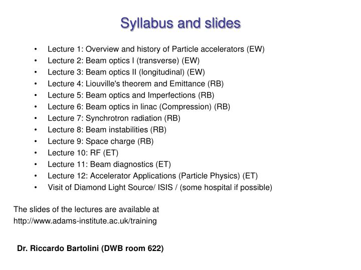
Syllabus and slides. Lecture 1: Overview and history of Particle accelerators (EW) Lecture 2: Beam optics I (transverse) (EW) Lecture 3: Beam optics II (longitudinal) (EW) Lecture 4: Liouville's theorem and Emittance (RB) Lecture 5: Beam optics and Imperfections (RB)

E N D
Syllabus and slides Lecture 1: Overview and history of Particle accelerators (EW) Lecture 2: Beam optics I (transverse) (EW) Lecture 3: Beam optics II (longitudinal) (EW) Lecture 4: Liouville's theorem and Emittance (RB) Lecture 5: Beam optics and Imperfections (RB) Lecture 6: Beam optics in linac (Compression) (RB) Lecture 7: Synchrotron radiation (RB) Lecture 8: Beam instabilities (RB) Lecture 9: Space charge (RB) Lecture 10: RF (ET) Lecture 11: Beam diagnostics (ET) Lecture 12: Accelerator Applications (Particle Physics) (ET) Visit of Diamond Light Source/ ISIS / (some hospital if possible) The slides of the lectures are available at http://www.adams-institute.ac.uk/training Dr. Riccardo Bartolini (DWB room 622)
Lecture 4: Emittance and Liouville’s theorem Hill’s equations (recap) More on transfer matrix formalism Courant-Snyder Invariant Emittance Liouville’s theorem
Linear betatron equations of motion (recap) In the magnetic fields of dipoles magnets and quadrupole magnets the coordinates of the charged particle w.r.t. the reference orbit are given by the Hill’s equations weak focussing of a dipole quadrupole focussing No periodicity is assumed but for a circular machine Kx, Kz and are periodic These are linear equations (in y = x, z). They can be integrated.
Pseudo-harmonic oscillations (recap) The solution can be found in the form which are pseudo-harmonic oscillations The beta functions (in x and z) are proportional to the square of the envelope of the oscillations The functions (in x and z) describe the phase of the oscillations
The solutions of the Hill’s equation can be cast equivalently in the form of principal trajectories. These are two particular solutions of the homogeneous Hill’s equation Principal trajectories (recap) which satisfy the initial conditions C(s0) = 1;C’(s0) = 0; cosine-like solution S(s0) = 0;S’(s0) = 1; sine-like solution The general solution can be written as a linear combination of the principal trajectories
We can express amplitude and phase functions Principal trajectories vs pseudo harmonic oscillations in terms of the principal trajectories Simple algebraic manipulations yield and viceversa or more simply
As a consequence of the linearity of Hill’s equations, we can describe the evolution of the trajectories in a transfer line or in a circular ring by means of linear transformations Principal trajectories (recap) C(s) and S(s) depend only on the magnetic lattice not on the particular initial conditions This allows the possibility of using the matrix formalism to describe the evolution of the coordinates of a charged particles in a magnetic lattice
Transfer lines or circular accelerators are made of a series of drifts and quadrupoles for the transverse focussing and accelerating section for acceleration. Each of these element can be associated to a particular transfer matrix Matrices of most common elements Matrix of a drift space Thin lens approximation L 0, with KL finite Matrix of a focussing quadurpole Matrix of a defocussing quadurpole
For each element of the transfer line we can compute, once and for all, the corresponding matrix. The propagation along the line will be the piece-wise composition of the propagation through all the various elements Q1 Q2 L Matrix formalism for transfer lines s1 s2 Notice that it works equally in the longitudinal plane, e.g. thin lens quadrupole associate to an RF cavity of voltage V and length L
Particle trajectories can be described with a matrix formalism analogous to that describing the propagation of rays in an optical system. Matrix formalism and analogy with geometric optics Magnetic field of a quadrupole and Lorentz force The magnetic quadrupoles play the role of focussing and defocussing lenses, however notice that, unlike an optical lens, a magnetic quadrupole is focussing in one plane and defocussing in the other plane.
Consider an alternating sequence of focussing (F) and defocussing (D) quadrupoles separated by a drift (O) A slightly more complicated example: the FODO lattice (I) The transfer matrix of the basic FODO cell reads
Matrix elements from principal trajectories and optics functions In terms of the amplitude and phase function the transfer matrix will read where 0 , 0 and the phase 0 are computed at the beginning of the segment of transfer line We still have not assumed any periodicity in the transfer line. If we consider a periodic machine the transfer matrix over a whole turn reduces to (put = the phase advance in one turn) This is the Twissparameterisation of the one turn map
Stability of motion with the matrix formalism Consider a circular accelerator with transfer matrix over one turn equal to M (one turn map). Using the Twissparameterisation for M After n turns, the transformation of the particle coordinates will be given by the successive application of the one turn matrix n times In order for the phase advance to be real and hence for the motion to be a stable oscillation, the one turn map must satisfy the condition It can be proven that (see bibliography)
Using the Twissparameterisation of the matrix or the FODO cell we have Example: the FODO lattice (II) hence The stability requires In a similar way we can compute the optics functions at the beginning of the FODO cell.
While in a circular machine the optics functions are uniquely determined by the periodicity conditions, in a transfer line the optics functions are not uniquely given, but depend on their initial value at the entrance of the system. We can express the optics function in terms of the principal trajectories as Optics functions in a transfer line This expression allows the computation of the propagation of the optics function along the transfer lines, in terms of the matrices of the transfer line of each single element, i.e. also the optics functions can be propagated piecewise from
In a drift space Examples The function evolve like a parabola as a function of the drift length. In a thin focussing quadrupole of focal length f = 1/KL The function evolve like a parabola in terms of the inverse of focal length
Diamond LINAC to booster transfer line Booster optics functions at the injection point Optics functions from the LINAC (Twiss parameters of the beam)
The solution of the Hill’s equations Betatron motion in phase space (recap) describe an ellipse in phase space (y, y’) area of the ellipse in phase space (y, y’) is
Hill’s equations have an invariant Courant-Snyder invariant (I) This invariant is the area of the ellipse in phase space (y, y’) multiplied by . This can be easily proven by substituting the solutions y, y’ into A(s). You will get the constant A(s) is called Courant-Snyder invariant
Whatever the magnetic lattice, the area of the ellipse stays constant (if the Hill’s equations hold) At each different sections s, the ellipse of the trajectories may change orientation shape and size but the area is an invariant. Courant-Snyder invariant (II) This is true for the motion of a single particle !
A beam is a collection of many charged particles The beam occupies a finite extension of the phase space and it is described by a distribution function such that Real beams – distribution function in phase space The beam distribution is characterised by the momenta of various orders Average coordinates (usually zero) The R-matrix also called -matrix describes the equilibrium properties of the beam giving thesecond order momenta of the distribution R11 = bunch H size; R33 = bunch Y size; R55 bunch Z size; R66 = energy spread
In many cases the equilibrium beam distribution is a Gaussian distribution Gaussian beams Usually the three planes are independent hence in each plane The isodensity curves are ellipses
The 6x6 –matrix can be partitioned into nine 2x2 submatrices with (assuming <x> = 0 and <x’> = 0) -matrix for Gaussian beams Direct computation using yields We can associate an ellipse with the Gaussian beam distribution. The evolution of the beam is completely defined by the evolution of the ellipse The ellipse associated to the beam is chosen so that its Twiss parameters are those appearing in the distribution function, hence, e.g.
For a generic beam described by a distribution functions we can still compute the average size and divergence and the whole -matrix Generic beams – rms emittance we associate to this distribution the ellipse which has the same second order momenta Rij and we deal with this distribution as if it was a Gaussian distribution and since The invariant of the ellipse will be which is the rms emittance of the beam
We have seen that the beam distribution can be associated to an ellipse containing 66% of the beam (one r.m.s.) In this way the beam rms emittance is associated with the Courant Snyder invariant of the betatron motion Beam emittance and Courant-Snyder invariant This links a statistical property of the beam (rms emittance) with single particle property of motion (the Courant-snyder invairnat) In this way the Courant-Snyder invariant acquires a statistical significance as rms emittance of the beam. Hence the beam rms emittance is a conserved quantity also for generic beams. This is valid as long as the Hill’s equations are valid or more generally the system is Hamiltonian. As such the conservation of the emittance is a manifestation of the general theorem of Hamiltonian system and statistical mechanics known as the Liouville theorem
Liouville’s theorem: In a Hamiltonian system, i.e. n the absence of collisions or dissipative processes, the density in phase space along the trajectory is invariant’. Liouville’s theorem Liouville theorem states that volume of 6D phase are preserved during the beam evolution (take f to be the characteristic function of the volume occupied by the beam). However if the Hamiltonian can be separated in three independent terms The conservation of the phase space density occurs for the three projection on the (x, px) plane (Horizontal emittance) (y, py) plane (Vertical emittance) (z, pz) = (, ) plane (longitudinal emittance)
The Courant-Snyder invariant is the area of the ellipse phase space. The conservation of the area is a general property of Hamiltonian systems (any area not only ellipses !) The invariance of the rms emittance is the particular case of a very general statement for Hamiltonian systems (Liouville theorem) This is valid as long as the motion is Hamiltonian, i.e. No damping effects, no quantum diffusion, due to emission of radiation no scattering with residual gas, no beam beam collisions no collective effects (e.g. interaction with the vacuum chamber, no self interaction) Beam emittance and Liouville’s theorem
E. Wilson, Introduction to Particle Accelerators J. Rossbach and P. Schmuser, CAS Lecture 94-01 K. Steffen, CAS Lecture 85-19 Bibliography