Download
1 / 28
280 likes | 469 Views
CMB and varying constants: T CMB (z) from SZE. Gemma Luzzi Experimental Cosmology Group Dept. of Physics - University of Rome “La Sapienza”. Workshop “ Varying Fundamental Constants ” Lorentz Center, Le iden, 18 May - 20 May 2009. Outline. CMB and varying constants

E N D
CMB and varying constants: TCMB(z)from SZE Gemma Luzzi Experimental Cosmology Group Dept. of Physics - University of Rome “La Sapienza” Workshop “Varying Fundamental Constants” Lorentz Center, Leiden, 18 May - 20 May 2009
Outline • CMB and varying constants • TCMB(z): why measure it? • SZE • TCMB(z) from SZE • SZE experiments
Cosmic Microwave Background (CMB) The CMB is the dominant radiation field in the Universe. Discovered in 1965 by Penzias and Wilson. One of the most powerful pieces of informations in support of Big Bang theory. The Big Bang theory (Gamov 1948) foresees a primordial Universe which expands while cooling down. The early Universe can be described as a plasma, in which ionized matter is coupled to radiation through Thomson scattering. When the temperature falls below 3000K (at z1000) electrons and protons recombine forming neutral hydrogen. Thomson scattering is no longer effective, therefore matter and radiation decouple. The mean free path of photons becomes larger than the causal horizon: photons can travel freely to us. Being the CMB generated in a thermal equilibrium state, we expect a blackbody spectrum. Observations by FIRAS on board COBE satellite have confirmed that the radiation is extremely close to the black body form at a temperature T0 = (2.7250.002)K The CMB is interpreted as an image of the Universe at decoupling, that is the image of the surface from which photons were scattered by electrons for the last time.
CMB and varying constants The inhomogeneities in the matter distribution at z=1000 produced intensity fluctuations of the radiation field: Primary Anisotropies. Predicted anisotropies are very sensitive to a wide range of cosmological parameters: accurate measurements of them provide excellent constraints on cosmological models. Changing the fine structure constant modifies the strenght of the electromagnetic interaction and thus the only effect on CMB anisotropies arises from the change in the differential optical depth of photons due to Thomson scattering WMAP TT cross power spectrum Changing EM has two effects: • changes the temperature at which the last scattering happens • changes the residual ionization after recombination First dependence on fine structure constant EM Both effects influence the CMB temperatures anisotropies: increasingEMpushes the last scattering surface at higher redshift thus leading to a smaller sound horizon at decoupling (larger lpeak). The second effect results from a smaller Silk Damping (increases the power on very small scales). (Uzan, Rev. Mod. Phys. 75, (2003)) (Martins et al. Physletb 2004)
CMB and varying constants The inhomogeneities in the matter distribution at z=1000 produced intensity fluctuations of the radiation field: Primary Anisotropies. Predicted anisotropies are very sensitive to a wide range of cosmological parameters: accurate measurements of them provide excellent constraints on cosmological models. Changing the fine structure constant modifies the strenght of the electromagnetic interaction and thus the only effect on CMB anisotropies arises from the change in the differential optical depth of photons due to Thomson scattering (Fig. by S. Galli) Changing EM has two effects: • changes the temperature at which the last scattering happens • changes the residual ionization after recombination First dependence on fine structure constant EM Both effects influence the CMB temperatures anisotropies: increasingEMpushes the last scattering surface at higher redshift thus leading to a smaller sound horizon at decoupling (larger lpeak). The second effect results from a smaller Silk Damping (increases the power on very small scales). (Uzan, Rev. Mod. Phys. 75, (2003)) (Martins et al. Physletb 2004)
CMB and varying constants The inhomogeneities in the matter distribution at z=1000 produced intensity fluctuations of the radiation field: Primary Anisotropies. Predicted anisotropies are very sensitive to a wide range of cosmological parameters: accurate measurements of them provide excellent constraints on cosmological models. Changing the fine structure constant modifies the strenght of the electromagnetic interaction and thus the only effect on CMB anisotropies arises from the change in the differential optical depth of photons due to Thomson scattering (Fig. by S. Galli) Changing EM has two effects: • changes the temperature at which the last scattering happens • changes the residual ionization after recombination First dependence on fine structure constant EM Both effects influence the CMB temperatures anisotropies: increasingEMpushes the last scattering surface at higher redshift thus leading to a smaller sound horizon at decoupling (larger lpeak). The second effect results from a smaller Silk Damping (increases the power on very small scales). (Uzan, Rev. Mod. Phys. 75, (2003)) (Martins et al. Physletb 2004)
TCMB(z): why measure it? • Observational test of the standard model: TCMB(z)=T0(1+z) T0 = (2.7250.002)Ksolar system value measured by COBE/FIRAS(Mather et al.1999) • Test of the nature of redshift (test of the Tolman’s law(Tolman. R. C., 1930, Proc. Nat. Acad, Sci., 16, 511) ) ; Sandage 1988; Lubin & Sandage 2001) • Constraints on alternative cosmological models (which rely on the physics of the matter and radiation content of the Universe): • -decaying models (Overduin and Cooperstock, Phys.Rev.D, 58 (1998)); (Puy,A&A,2004); (Lima et al., MNRAS, 312 (2000)) • Decaying scalar field cosmologies • Possible constraints on the variation of fundamental constants over cosmological time
TCMB(z): measurements Measurements of CMB temperature traditionally through the study of excitation temperatures in high redshift molecular clouds. First attempt pionered by (Bahcall and Wolf, 1968) • Many high redshift estimates of TCMB at redshift of absorbers (Songaila et al 1994; Lu et al. 1996; Ge et al 1997; Roth and Bauer, 1999; Srianand et al 2000; loSecco et al. 2001; Levshakov et al. 2002; Molaro et al. 2002; Cui et al. 2005) • Systematics: • CMB is not the only radiation field populating the energy levels, from which transitions occur. • detailed knowledge of the physical conditions in the absorbing clouds is necessary (Combes and Wiklind, 1999; Combes ,2007) (LoSecco et. Al. Phys. Rev. D, 64, 123, 2002)
The Sunyaev Zel’dovich Effect (SZE) (I) Secondary CMB anisotropy Comptonization of the CMB by electrons in the hot gas of galaxy clusters. SZE = SZTERM + SZCIN + SZCOR REL R function= relativistic corrections (Rephaeli 1995-Itoh et al. ApJ 502, 7, 1998 – Shimon & Rephaeli ApJ 575, 12, 2002)
Properties: unique spectral shape Redshift independent electron pressure in cluster atmospheres The Sunyaev Zel’dovich Effect (SZE) (II) (Carlstrom JE A&A, 40, 643, 2002) Xrays Xrays Xrays Spectral distorsion of the CMB due to the SZE (Carlstrom JE A&A , 40, 643,2002) • Cosmology: • H0 • B • evolution of abundance of clusters • TCMB(z) • Galaxy clusters Physics: • optical depth • Te electronic temperature • vpec peculiar velocity
TCMB(z) from SZE (I) (Fabbri R., F. Melchiorri & V. Natale. Ap&SS 59, 223, 1978; Rephaeli Y. Ap.J. 241, 858, 1980) ISZdepends on frequency through the nondimensional ratio h/kT: redshift-invariant only for standard scaling of T(z) In all other non standard scenarios, the “almost” universal (remember rel. corrections!) dependence of thermal SZ on frequency becomes z-dependent, resulting in a small dilation/contraction of the SZ spectrum on the frequency axis. Ex: TCMB(z) = TCMB(0)(1+z)1-a (Lima et al. 2000) T*CMB= TCMB(0)(1+z)-a where
TCMB(z) from SZE (II) • Steep frequency dependency of ISZ TCMB(z) • Ratio of ISZ(1)/ISZ(2) weakly dependent on cluster properties (, Te, vpec) Relative variation of SZ signal, evaluated for a typical 10-4 comptonization parameter at a Te=10keV, Vpec=300km/s along l.o.s. Fig. by L. Lamagna
COMA observations SZ on A1656 by MITO OVRO + MITO (De Petris M. et al. Ap.JL 574, 119-122, 2002 & Savini G. et al. New Astr. 8, 7, 727-736, 2003) Complete SZ spectrum of COMA SZ on A1656 by OVRO+WMAP+MITO First SZ spectrum with 6 frequencies (Battistelli, et al. Ap.JL 2003)
TCMB(z) from SZE: first application Fit of measured SZ signals ratios with the expected values by changing T(z)/(1+z) as in the following: Gi : Responsivity Ai:Throughput i() :Transmission efficiency • independent of absolute calibration uncertainties (Tplanet); • independent of , if KIN-SZ removed or negligible; • dependent on precise knowledge of Ai and i() • Ratios have non gaussian distributions and introduce correlations
TCMB(z) from SZE: first results COMA+A2163 OVRO+BIMA+SuZIE OVRO+MITO COBE • Lo Secco et al. 2001 Molaro et al. 2002 Molecular microwave transitions CONSISTENT Standard Model CONSISTENT (Battistelli et al., ApJL 580, 101, 2002)
TCMB(z) from SZE: extended dataset SZ measurements of 14 clusters by different experiments expressed in central thermodynamic temperature X-ray data (Bonamente et al., APJ,647,25,2006) (De Gregori et al. Nuovo Cimento B, 122, 2008)
Joint likelihood to extract the universal parameter “a” of the Lima model • Ratios of SZ intensity change (RI) ISZ(1)/ISZ(2) • weakly dependent on IC gas properties if negligible. • Joint likelihood to extract the universal parameter “a” of the Lima model • single likelihoods for each cluster to provide individual determinations of TCMB(z) at z of each cluster • independent from the particular scaling assumed for the temperature (i.e. the Lima model) • only assumption (z)=0(1+z) • Directly ISZmeasurements (DI) • easier control of systematics • more complex structure in the parameter space TCMB(z) from SZE: improved statistical analysis Two main approaches: Priors: P(Tei) = N(E(Tei),(Tei)) P(vp) = N(0 km/s,1000 km/s) P(TCMB) = flat P() = flat (only for DI) P(C) = N(1,0.1) (Luzzi et al. in preparation)
TCMB(z) from SZE: Ratios approach (RI) Likelihood of intensity ratios: • weak dependence on cluster parameters (no marginalization on ) • not considered measurements at the crossover frequency (Cauchy tail) • bias due to arbitrariness in selecting the intensity change used in denominator of ratios • more precise SZ measurements or larger dataset bias removed Probability function for ratio r: Two measurements 1 e 2with gaussian errors 1 e 2: Extended to the case of n ratios
TCMB(z) from SZE: Direct approach DI multicluster likelihood: (numerical integration, integration analytical) P(d|a,,Te,vp,C) = iP(di|a,,Te,vp,C) P(a|d) P(d|a,,Te,vp,C) P(a)P()P(Te)P(vp)P(C)d dTe dvpdC DI single likelihood for each cluster: • MCMC algorithm • (Metropolis-Hastings sampling; • Gelman-Rubin test for convergence ) • Posteriors for all parameters • Study of correlations • Main degeneracies: • T(z) vs • T(z) vs vpalways evident
TCMB(z) from SZE: Results Flat prior a [0,1] (theoretical motivation) (Lima et al 2000) All limits are at 68% probability level RI a 0.092 DI (JL) a 0.059 DI (SL-MCMC) a 0.12 (including lines a 0.079) From lines transition observations Consistency with std. Model Posterior for “a”
TCMB(z) from SZE: simulations Simulated observations of 50 well known clusters mock dataset analyzed to recover input parameters of the cluster Analysis: MCMC allows to explore the full space of the cluster parameters and the TCMB(z) P(vp) = N(0 km/s,1000 km/s) P(vp) = N(0 km/s,100 km/s) P(Te) = N(6.50KeV,0.14KeV )
SZE experiments • Ongoing and near future surveys with ACT, APEX-SZ, SPT, Planck and detailed mapping of a sample of nearby clusters with MAD and OLIMPO experiments will provide much more precise and uniform datasets: • bias in the ratio approach largely removed • reduced skweness in and Tcmb(z)distributions (DI)
MAD MITO(Millimeter and Infrared Testagrigia Observatory) MAD (Multi Array of detectors) photometer upgrades MITO with a multi-pixel configuration based on bolometer array consisting of 3x3 pixels operating at four frequency bands (142, 217, 269, 353 GHz) and with beamsizes down to 4.5’. 142 GHZ 217 GHZ 269 GHZ 353 GHZ (Lamagna, et al., 2004 Proc of Enrico Fermi School, CLIX. SIF, 2005)
Planned observations • 47 simulated well known galaxy clusters (from BAX catalog) observed in 4 frequency bands with angular resolution ranging from 4.7 and 1.9 arcmin. • Assumed atmosphere noise with 90% transparency. • “Blind” data treatment and signal extraction • MCMC to fit on SZ parameters+CMB temp. (Sims and fit by L. Lamagna)
Future SZE experiments • Accurate spectroscopic observations from space towards a limited number of clusters (like the proposed SAGACE satellite) would allow to control a large part of the degeneracies between TCMB(z) and cluster parameters.
SAGACE project SAGACE (Spectroscopy Active Galaxies and Clusters Explorer) • Space borne spectrometer, coupled to a 3m telescope: • able to cover frequency ranges 100-450 and 720-760 GHz, • With angular resolution ranging from 4.2 to 0.7 arcmin • with photon noise limited sensitivity • The SAGACE observational program aims at performing a millimetric and submillimetric spectroscopy study from space of cosmic structures in the Universe. • SAGACE will provide spatially resolved spectroscopic observations of clusters with exquisite precision and accuracy.
Scientific impact of SAGACE The high accuracy of the spectral measurements allows to control a large part of the existing degeneracies between the cluster parameters. SAGACE SAGACE 3BP Planck SAGACE SAGACE 3BP 3BP Planck
Conclusions • Original tool to observationally test the standard scaling of TCMB and its isotropy up to the redshift of galaxy clustersand to put constraints on alternative cosmological models. • With near future SZE experiments more precise measurements of the TCMB(z) scaling law could set constraints on the variation of fundamental constants over cosmological time.