Download
1 / 39
390 likes | 496 Views
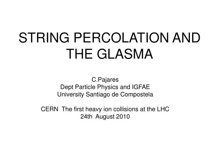
STRING PERCOLATION AND THE GLASMA. C.Pajares Dept Particle Physics and IGFAE University Santiago de Compostela CERN The first heavy ion collisions at the LHC 24th August 2010. Introduction to percolation of strings Results for some observables Similarities on rapidity distributions,and

E N D
STRING PERCOLATION AND THE GLASMA C.Pajares Dept Particle Physics and IGFAE University Santiago de Compostela CERN The first heavy ion collisions at the LHC 24th August 2010
Introduction to percolation of strings • Results for some observables • Similarities on rapidity distributions,and multiplicity distributions . Behaviour of normalized width with energy or density . Long range correlations . EoS J.Dias de Deus.EoS(B.Srisvastava,et al)
= E 0.2 0.9 2.36 dN/dy 2.75 3.48 4.47 Pt 0.40 0.46 0.50 Pt**2/dN/dy 0.058 0.060 0.056 LHC
The STAR analysis of charged hadrons for 0 to 10% central Au+Au collisions at √sNN =200 GeV gives a value η =2.88 ± 0.09 [8]. Above the critical value of η the QGP in SPM consists of massless constituents (gluons). The connection between η and the temperature T(η) involves the Schwinger mechanism (SM) for particle production. In CSPM the Schwinger distribution for massless particles is expressed in terms of pt2 (9) with the average string tension value < x2 >. Gaussian fluctuations in the string tension around its mean value transforms SM into the thermal distribution [6] (10) with <x2>= π <pt2>1/F(η). The temperature is given by (11) where F(η) and <pt2>1can be obtained from the data as described above. 22
The dynamics of massless particle production has been studied in QE2 quantum electrodynamics. QE2 can be scaled from electrodynamics to quantum chromodynamics using the ratio of the coupling constants. The production time τprofor a boson (gluon) is (18) For mc2we use <mt> andτpro= 1.128 ± 0.009 fm/c. This gives εi= 2.27±0.16 GeV/fm3at η=2.88. In SPM the energy density εat y=0 is proportional to η. From the measured values of ηand ε it is found that ε is proportional to η for the range 1.2 < η < 2.88 [8, 15]. εi = 0.788 η C Y. Wong, Introduction to high energy heavy ion collisions, 289 (1994). J. Schwinger, Phys. Rev. 128, 2425 (1962). 24
This relationship (19) has been extrapolated to below η = 1.2 and above η= 2.88 for the energy and entropy density calculations. Figure 1 shows ε/T4 obtained from SPM along with the LQCD calculations . The number of degrees of freedom G(T) are: At Ti , εi = 2.27 ± 0.16 GeV/fm3 and 37.5 ± 3.6. DOF At Tc, εC = 0.95 ± 0.07 GeV/fm3 and 27.7±2.6 DOF. 25
FIG: The energy density from SPM versus T/TSPM (red circles) and Lattice QCD energy density vs T/TLQCD (blue dash line) for 2+1 flavor and p4 action. 26
(12) (13) (14) (15) (16) where ε is the energy density, s the entropy density, τ the proper time, and Cs the sound velocity. Above the critical temperature only massless particles are present in SPM. Bjorken 1D Expansion and the velocity of sound in the QGP 27
FIG: The speed of sound from SPM versus T/TC CSPM (red circles) and Lattice QCD-p4 speed of sound versus T/TC LQCD (blue dash line) . The physical hadron gas with resonance mass cut off M ≤ 2.5 GeV is shown ( green circles). 28
FIG. : The energy density from SPM versus T/TSPM (red circles) and Lattice QCD energy density vs T/TLQCD (blue dash line) for 2+1 flavor and p4 action. 3p/T4 is also shown for SPM (green circles). 29
FIG. : The entropy density from SPM versus T/TCCSPM (red circle) and Lattice QCD entropy density versus T/TC LQCD(blue dash line) . 30
The determination of the EOS of hot, strongly interacting matter is one of the main challenges of strong interaction physics (Hot QCD Collaboration) . Recently, Lattice QCD (LQCD) presented results for for the bulk thermodynamic observables, e.g. pressure, energy density, entropy density and for the sound velocity. We use SPM to calculate these quantities and compare them with the LQCD results. The QGP according to SPM is born in local thermal equilibrium because the temperature is determined at the string level. After the initial temperature TI >Tc , SPM may expand according to Bjorken boost invariant 1D hydrodynamicS A. Bazavov et al, Phys. Rev. D80 (2009) 014504 37
The sound velocity requires the evaluation of s and dT/dε , which can be expressed in terms of ηand F(η). With q1/2 = F(η) one obtains: Then CS2 becomes: CS2 = (1+CS2) (−0.25) for η ≥ ηC (22) An analytic function of η for the equation of state of the QGP for T ≥ Tc . Figure shows the comparison of CS2from SPM andLQCD. The LQCD values were obtained using the EOSof 2+1 flavor QCD at finite temperature with physicalstrange quark mass and almost physical light quarkmasses [14]. At T/Tc=1 the SPM and LQCD values agree withthe CS2 = 0.14 value of the physical hadron gas with resonancemass truncation M ≤ 2.5 GeV P. Castorina et al, arXiv:hep-ph/0906.2289v1 38