Download
1 / 77
770 likes | 890 Views
Explore the groundbreaking Anatomic Gene Expression Atlas (AGEA) created by the Quantitative Neuroscience Laboratory at Boston University. This cutting-edge atlas includes detailed reconstructions, structural annotations, and gene expression profiles of the brain. Learn how In Situ Hybridization (ISH) techniques provide vital spatial information on gene expression, leading to a deeper understanding of cellular phenotypes and brain function. Discover the reproducibility and data processing techniques used in this innovative research. Access a wealth of information on the Allen Reference Atlas and the ontology used for data labeling. Dive into the specifics of gene expression statistics, data normalization, and expression energy calculations, all contributing to a comprehensive neuroscientific resource.

E N D
A Big Thanks Prof. Jason Bohland Quantitative Neuroscience Laboratory Boston University
The Process Construction and representation of the Anatomic Gene Expression Atlas (AGEA).
Allen Reference Atlas • 3D Nissl volume comes from rigid reconstruction • Each section reoriented to match adjacent images as closely as possible • A 1.5T low resolution 3D average MRI volume used to ensure reconstruction is realistic • Reoriented Nissl section down-sampled, converted to grayscale • Isotropic 25μm grayscale volume.
Anatomy • 208 large structures and structural groupings extracted • Projected & smoothed onto 3D atlas volume to for structural annotation • Additional decomposition of cortex into an intersection of 202 regions and areas
The Process Construction and representation of the Anatomic Gene Expression Atlas (AGEA).
Coronal section Sagittal section InSitu Hybridization or ISH Each gene ISH series is reconstructed from serial sections (200 μm spacing)
Why ISH ? • Phenotypic properties in cells result of unique combination of expressed gene products • Gene expression profiles => define cell types.
6 genes on 1 brain • Each gene on 56 sections • 2 sections are forNissl
8 genes on 1 brain • Each gene on 20 Sections.
ISH – Tissue Preparation & Imaging Process • Sectioning • Staining (Non-isotopic digoxigenine (DIG)) • Washing • Imaging
Traditional Approach vs. ISH • in situ hybridization measures expression & preserves spatial information for single gene • Finer resolution – • cellular but not single cell • Data can be used to analyze • Gene expression • Gene regulation • CNS function (spatial) • Cellular phenotype (spatial) • Histology • One gene at a time • For 20,000 genes need 20000 x (5 or 14) slides ~1year • DNA microarrays & SAGE - Applied to large brain region • Cannot differentiate neuronal subtypes Kamme, F et. al. J. Neurosci (2003) Sugino, K. et. al. Nature Neurosci (2006)
Reproducibility For multiple genes, inbred mouse strain used Although different mice used for different genes, expression for under same environmental conditions are reproducible.
Is ISH Reproducible? • Primary Source of variation comes from • Riboprobes • Day-to-day variability • Biological variability in brains • Still with inbred mice, variation between brains is significant.
Processing Expression Statistics Reconstruction – 3D Data accessed by standard coord system – 200^3 μmvoxels Ontology of Allen Reference Atlas used to label individual voxels
Grid Based Nearest Plane
Registration - Key • Volumes iteratively registered to AB atlas using affine and locally nonlinear warping • Registration good to ~200 microns Local deformation field example
Lower dimensional data volumes • Analyze binnedexpression volumes at 200 µm3 resolution • ~31,000 image series (mostly single hemisphere, sagittal series) • 4,104 unique genes available from coronally sectioned brains • Each volume is 67 x 41 x 58 voxels (about 50k brain voxels) • Comparable to fMRI resolution
Data normalization • Background correction & Registration • Intensity normalization – • Correct background from negative control • Registration - • Map the image to the reference atlas • Smoothed Expression Energy • Sum of intensities of expressing cells / # of cells in the voxel • An average over many cells of diverse types
ISH Signal (c) Coronal plane in situ hybridization (ISH) image of gene tachykinin 2 (Tac2) from the Allen Brain Atlas showing enriched expression in the bed nucleus of the striaterminalis (BST). The box represents a 1-mm2 square. (d) Enlarged expression mask view of boxed area in c depicting gene expression levels color coded by ISH signal intensity (red, higher expression level; green/blue, lower expression level).
Measurements p is a image pixel invoxel C |C| is the total number of pixels in C M(p) - expression segmentation mask 1 (“expressing” pixel) or 0 (“non expressing” pixel) I(p) grayscalevalue of ISH image intensity Gray = 0.3*Red + 0.59*Green + 0.11*Blue.
Prox1 volume maximum intensity projections Coronal section Sagittal section Per Gene Signature Prox1 Raw ISH Expression Energy
Recap - Measurements Expression measures • expression density = sum of expressing pixels / sum of all pixels in division • expression intensity = sum of expressing pixel intensity / sum of expressing pixels • expression energy = sum of expressing pixel intensity / sum of all pixels in division • == density x intensity
MetaData • Each voxel can be connected to a node in a hierarchical brain atlas / ontology, and also to Waxholmspace • Raw Nissl sections from the same brain (with 200 μm spacing) can also be obtained • Each gene has specific probe sequence used, various identifiers to link to gene information (we’ve used Entrez ID)
Large-scale data analysis • How much structure is present across space and across genes? • How would the brain segment on the basis of gene expression patterns (as opposed to Nissl, etc.)? • Is there structure in the patterns of expression of highly localized genes? • What can we learn from the expression patterns of genes implicated in disorders? see Bohland et al. (2009) Methods; Ng et al. (2009) Nature Neuroscience.
Genome-wide Analysis of Expression 70.5% genes expressed in less than 20% cells
Notes • Well-established genes for different cells identified • For 12 major brain regions, 100 top genes.
Cell-Specific Genes Gene Ontology enrichment analysis useful Oligodendrocyte-enriched genes => myelin production.
Functional Compartments Genes with regional expression provides substrates for functional differences
Tools from AGEA • Correlation mode – View navigate 3-D spatial relationship maps • Clusters mode – Explore transcriptome based spatial organization • Gene Finder mode - Search for genes with local regionality
Spatial Transcriptome • Expression energy for each gene (M=4,376) and for each voxel (N=51,533) • For each voxel • find Pearson’s correlation coefficient between seed voxel and other voxel using expression vectors of length M • Compute 51,533 three-dimensional correlation maps • Web viewer for easy navigation between maps and within each 3-D map • Correlation values as 24-bit false color using a blue-to-red (“jet”) color scale
Clusters of Correlated Gene Expression • Classical definition of brain regions • Overall Morphology • Cellular Cytoarchitecture • Ontological Development • Functional Connectivity
Clusters of Correlated Gene Expression • Hierarchical clustering – • Voxels are spatially organized as a binary tree • Each node is collection of voxels and has 0 or 2 branches • Initially 51,533 voxels assigned to root node of the tree. • Final tree has103,065 nodes with a maximum depth of 53 levels and 51,533 leaf nodes (one for each voxel in the brain). • At each bifurcation an ordering is assigned to each child to enable the definition a global “depth first” ordering for all leaf nodes.
Microarray Data Analysis K-means Hierarchical Clustering Biclustering CLICK Self-Organizing Maps DBSCAN OPTICS DENCLUE … Statistical Analysis Unsupervised Analysis – clustering Supervised Analysis Pattern Analysis Visualization & Decomposition
Differentially Regulated Genes Up regulated genes Down regulated genes