Download
1 / 43
440 likes | 541 Views
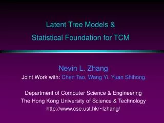
Search-based Learning of Latent Tree Models. Tao Chen Department of Computer Science & Engineering The Hong Kong University of Science & Technology. Y1. Y2. Y3. X4. X7. X1. X2. X3. X5. X6. Latent Tree Models (LTM). Bayesian networks with Rooted tree structure

E N D
Search-based Learning of Latent Tree Models Tao Chen Department of Computer Science & Engineering The Hong Kong University of Science & Technology
Y1 Y2 Y3 X4 X7 X1 X2 X3 X5 X6 Latent Tree Models (LTM) • Bayesian networks with • Rooted tree structure • Discrete random variables • Leaves observed (manifest variables) • Internal nodes latent (latent variables) • Denoted by (m, θ) • m is the model structure • θ is the model parameters • Also known as hierarchical latent class (HLC)models, HLC models P(Y1), P(Y2|Y1), P(X1|Y2), P(X2|Y2), …
Example • Manifest variables • Math Grade, Science Grade, Literature Grade, History Grade • Latent variables • Analytic Skill, Literal Skill, Intelligence Intelligence Literal Skill Analytic Skill Math Grade Science Grade Literature Grade History Grade
Search-Based method • maximizing the BIC score: BIC(m|D) = max θ log P(D|m, θ) – d(m) logN/2 Y1 Y2 Y3 X4 Maximized loglikelihood Penalty X7 X1 X2 X3 X5 X6 Learning Latent Tree Models Observed Data: D • Number of latent variables • Cardinality (i.e. number of states) of each latent variable • Model Structure • Conditional probability distributions
Cluster Analysis • Cluster analysis • partitioning of objects into groups • objects in each group share some common trait • Classification of clustering methods • Latent Tree (LT) models
Y Literature Math Science History LT based clustering Intelligence Literal Skill Analytic Skill Math Science Literature History Multidimensional Clustering Weakness of LC clustering: • Local independence assumption is often violated • not a meaningful partition • Single dimension assumption: one way to partition data • not appropriate when a lot of attributes Clustering based on LT models: • Relax local independence • Multidimensional clustering • discover multiple ways to partition data in a single model LC based clustering
Outline • Introduction • Latent tree models • The problem of learning latent tree models • Motivation • Search-Based Algorithms • EAST Search • Three Issues • Operation Granularity • Range of Model Adjustment • Efficient Model Evaluation • New Algorithm: EAST_RR • Two-stage Model Evaluation • Comparison with the State-of-the-art • Multidimensional Clustering with LT models • Conclusion
X6 X7 X6 X7 X6 X7 Y2 Y2 X1 Y2 X1 X5 X1 X5 Y3 Y1 X2 Y3 X5 Y1 Y1 X2 X4 X2 X4 X3 X3 X4 X3 (a) m2 (a) m3 (a) m1 Search Operators • Expansion operators: • Node introduction (NI):m1 => m2 ; |Y3| = |Y1| • State introduction (SI):add a new state to a latent variable • Adjustment operator: node relocation (NR),m2 => m3 • Simplification operators: node deletion (ND),state deletion (SD)
Naïve Search • At each step: • Construct all possible candidate models by applying the search operators to the current model. • Evaluate them one by one (BIC) • Pick the best one • Complexity: • SI: O( l )l: the number of latent variables in the current model • SD: O( l ) • NR: O( l (l+n) )n: the number of manifest variables • NI: O( l r(r-1)/2 )r: the maximum number of neighbors (current) • ND: O( l r ) • Total : T = O( l ( 2 + r/2 + r2/2 + l + n) )
Reducing Number of Candidate Models • Reduce number of operators used at each step • How? BIC(m|D) =max θ log P(D|m, θ) – d(m) logN/2 • Three phases: • Expansion Phase: O( l (1 - r/2 + r2/2 ) ) < T • Search with expansion operators NI and SI • Improve the maximized likelihood term of BIC • Simplification Phase: O( l (1+r) ) < T • Search with simplification operators ND and SD, separately • Reduce penalty term • Adjustment Phase: O( l (l+n) ) < T • Search with adjustment operators NR • Restructure
EAST Search • Start with a simple initial model • Repeat until model score ceases to improve • Expansion Phase (NI, SI) • Adjustment Phase (NR) • Simplification Phase (ND, SD) • EAST: Expansion, Adjustment, Simplification until Termination
Outline • Introduction • Search-Based Algorithms • EAST Search • Three Issues • Operation Granularity • Range of Model Adjustment • Efficient Model Evaluation • New Algorithm: EAST_RR • Two-stage Model Evaluation • Comparison with the State-of-the-art • Multidimensional Clustering with LT models • Conclusion
2 2 2 3 … X1 … X2 X100 X100 X1 X2 … X1 X2 X100 Operation Granularity • Operation Granularity is raised in(Zhang & Kocka 2004) • Our contribution: • Empirical Study local maxima • Explanation to local maxima • Deal with the issue • Principle: Taking the size of the step into consideration • Empirically demonstrate the effectiveness m SI: 101 more parameters NI: 2 more parameters
Y1 … Y2 … … Y3 Y4 X2 X4 X5 X1 X3 … … … (a)m Y1 Y2 Y3 Y4 X2 X4 X5 X1 X3 (b) m1 Range of Model Adjustment Restricted NR • Adjustment: NR without restriction • Local Adjustment: Restricted NR (RNR) • Questions: • Which one: NR or Restricted NR • How often to adjust? • Extensive empirical study Adjustment (NR) + EAST … … … Y1 Y2 Y3 Y4 NR X2 X1 X4 X5 X3 (c) m2
Outline • Introduction • Search-Based Algorithms • EAST Search • Three Issues • Operation Granularity • Range of Model Adjustment • Efficient Model Evaluation • New Algorithm: EAST_RR • Two-stage Model Evaluation • Comparison with the State-of-the-art • Multidimensional Clustering with LT models • Conclusion
The Complexity of Model Evaluation • Compute likelihood term max θ log P(D|m, θ) in BIC • EM algorithm necessary because of latent variables • EM is an iterative algorithm • At each iteration, do inference for every data case l =30 the number of latent variables in the current model n =70 the number of manifest variables The complexity of EM algorithm has THREE factors • #of iterations: M = 100 • Sample size: N = 10,000 • Complexity of inference for one data case is the model size: O(l + n) • Evaluating a candidate model: O( MN(l + n) ) 108 • How to reduce the complexity: • Restricted Likelihood (RL) Method • Data Completion (DC) Method
Restricted Likelihood: Parameter Composition θ’1θ’2 θ1θ2 • m: current model; • m': candidate model generated by apply a search operator on m • The two models share many parameters • m: (θ1, θ2 ); m' : (θ1', θ2' ) Y1 Y1 Y2 Y3 Y2 Y3 Y4 X4 X4 X1 X5 X7 X1 X6 X7 X2 X3 X6 X2 X3 X5 (a) m (b) m’ (NI) old new
Restricted Likelihood • Know optimal parameter values for m: (θ1*, θ2*); • maximum restricted likelihood: • Freezing θ1' = θ1* and Varying θ2' • Likelihood ≈ Restricted Likelihood maxθ2' log P(D|m', θ1*, θ2' ) ≈ max(θ1', θ2' )log P(D|m', θ1', θ2' ) • RL based evaluation: likelihoodrestricted likelihood BIC_RL(m'|D) = maxθ2' log P(D|m', θ1*, θ2' ) – d(m') logN/2 • How the complexity is reduced? (sample size N = 10,000) • Need less iterations before convergence: M’ = 10 • Inference is restricted to new parameters: model size = O(1) M’N O(1) 105
Y Y Z W V W V (a) m (b) m’ Data Completion • Complete data D using(m, θ*) • Use to evaluate candidate models NI example • Null Hypothesis: • V and W are conditionally independent given Y • G-squared Statistic from • Model Selection • How the complexity is reduced? (sample size N = 10,000) • No iterations any more • Linear in sample size O(N) 104 (RL: 105)
RL vs. DC: Data Analysis • Two Algorithms: EAST-RL and EAST-DC • Date sets: • Synthetic data • Real-world data • Quality measurement: • Synthetic: empirical KL divergence (approximate); 10 runs • Real-world: logarithmic score on testing data (prediction); 5 runs
RL vs. DC: Efficiency • Synthetic data: • Real-world data:
RL vs. DC: Model Quality • Synthetic data: • 12 and 18 variables: EAST_RL beats EAST_DC • 7 variables: identical models • Real-world data: EAST_RL beats EAST_DC
Theoretical Relationships • Objective function: BIC functions • Resort to RL and DC due to hardness • How RL and DC are related to BIC? • Proposition 1 (RL and BIC) : For any candidate model m’ obtained from the current model m, RL functions ≤ BIC functions. • Proposition 2 (DC and BIC): For any candidate model m’ obtained from the current model m using the NR, ND or SD operator, DC functions (NR, ND and SD) ≤ BIC functions (NR, ND and SD) No clear relations between DC and BIC functions in the case of SI and NI operators.
Comparison of Function Values • RL functions • Tight lower bound BIC • DC functions • Lower bound BIC • Far away from BIC • Similar stories on ND, SD. large gap
Comparison of Function Values • RL functions: • Lower bound • Tight in most cases • Good ranking • DC functions: • Not lower bound • Bad ranking
Comparison of Model Selection • D7(1k), D7(5k), D7(10k) • RL and DC picked the same models • The other 6 data sets • Most steps : the same models • Quite a number of steps : RL picked better models.
Performance Difference Explained • EAST_RL uses RL functions in model evaluation • EAST_DC uses DC functions in model evaluation • RL functions are more closely related to BIC functions than DC functions • Theoretically • Empirically • Model Selection • RL picks better models than DC during search • EAST_RL finds better models than EAST_DC
Outline • Introduction • Search-Based Algorithms • EAST Search • Three Issues • Operation Granularity • Range of Model Adjustment • Efficient Model Evaluation • New Algorithm: EAST_RR • Two-stage Model Evaluation • Comparison with the State-of-the-art • Multidimensional Clustering with LT models • Conclusion
Model Evaluation Screening Evaluation Two-Stage Model Evaluation • Motivation: Speed up EAST_RL • Idea: Divide the evaluation into two stages • EAST_RR: is a shorthand of EAST_RL_RL • Both stages use RL • Screening stage: at low parameter setting • Evaluation stage: at high parameter setting
Comparison With the State-of-the-art • Previous State-of-the-art: HSHC (Zhang&Kocka 2004) • How EAST_RR compared with HSHC? • Synthetic data: • EAST_RR significantly more efficient than HSHC • EAST_RR find better models • D18(1k): 0.1865 (EAST_RR) < 0.3745 (HSHC) • D18(10k): 0.0044 (EAST_RR) < 0.0059 (HSHC) • Slightly better on the others data sets
Comparison With the State-of-the-art • Real-world data : • EAST_RR significantly more efficient than HSHC • EAST_RR find better models • New State-of-the-art: EAST_RR
Outline • Introduction • Search-Based Algorithms • EAST Search • Three Issues • Operation Granularity • Range of Model Adjustment • Efficient Model Evaluation • New Algorithm: EAST_RR • Two-stage Model Evaluation • Comparison with the State-of-the-art • Multidimensional Clustering with LT models • Conclusion
ICAC Data // 31 variables, 1200 samples C_City: s0 s1 s2 s3 // very common, common, uncommon, very uncommon C_Gov: s0 s1 s2 s3 // Ditto C_Bus: s0 s1 s2 s3 // Ditto Tolerance_C_Gov: s0 s1 s2 s3 //totally intolerable, intolerable, tolerable, totally tolerable Tolerance_C_Bus: s0 s1 s2 s3 WillingReport_C: s0 s1 s2 // yes, no, depends LeaveContactInfo: s0 s1 // yes, no I_EncourageReport: s0 s1 s2 s3 s4 // very sufficient, sufficient, average, ... I_Effectiveness: s0 s1 s2 s3 s4 //very e, e, a, in-e, very in-e I_Deterrence: s0 s1 s2 s3 s4 // very sufficient, sufficient, average, ... ….. -1 -1 -1 0 0 -1 -1 -1 -1 -1 -1 0 -1 -1 -1 0 1 1 -1 -1 2 0 2 2 1 3 1 1 4 1 0 1.0 -1 -1 -1 0 0 -1 -1 1 1 -1 -1 0 0 -1 1 -1 1 3 2 2 0 0 0 2 1 2 0 0 2 1 0 1.0 -1 -1 -1 0 0 -1 -1 2 1 2 0 0 0 2 -1 -1 1 1 1 0 2 0 1 2 -1 2 0 1 2 1 0 1.0 ….
Latent Structure Discovery Y2: Demographic info; Y3: Tolerance toward corruption Y4: ICAC performance; Y5: Change in level of corruption; Y6: Level of corruption Y7: ICAC accountability
Clusters in ICAC LT Model • ICAC LT model • latent variable partition • Y2(4): “Demographical Info” • Based on attributes {Sex, Age, Education, Income} • Y3(3): “Tolerance towards Corruption” • Based on attributes {tolerance_C_Bus, tolerance_C_Gov} • etc. • These people can be clustered in multiple ways (9 ways) • Multidimensional Clustering in a single model
Clustering Based on Y2 • The Class-Conditional Probability Distributions (CCPDs) for Y2 • Y2=s0: Low income youngsters; • Y2=s1: Women with no/low income; • Y2=s2: people with good education and good income; • Y2=s3: people with poor education and average income
Clustering Based on Y3 • The CCPDs for Y3 • Y3=s0: people who find corruption totally intolerable; 57% • Y3=s1: people who find corruption intolerable; 27% • Y3=s2: people who find corruption tolerable; 15%
Relationship between Y2 and Y3 • Interesting finding: Y2(DemoInfo) and Y3(tolerance toward corruption) • Y2=s2 (good education & good income): 4% tolerable the least tolerant • Y2=s3 (poor education & average income): 32% tolerable the most tolerant • The other two classes are in between.
Y … X1 X2 Xn LC Cluster Analysis • Latent class models • are a special class of Latent Tree models • contain a single latent variable • Learning an LC model • Start with an LC model with a binary latent variable Y • Repeat until no improvement • Increase |Y| by 1 • Compute BIC
… … ICAC Latent Class Model • Y is strongly related to 11 manifest variables • Meaning not clear: hard to interpret Y LC and LT cluster analysis • ICAC data (31 attributes) • naturally be partitioned in multiple ways • each way is based on a subset of attribute • LT cluster analysis can find these ways • multidimensional clustering; meaningful • LC cluster analysis force one way to cluster data • misguided, not meaningful
Outline • Introduction • Search-Based Algorithms • EAST Search • Three Issues • Operation Granularity • Range of Model Adjustment • Efficient Model Evaluation • New Algorithm: EAST_RR • Two-stage Model Evaluation • Comparison with the State-of-the-art • Multidimensional Clustering with LT models • Conclusion
Conclusion • EAST search framework • Three Issues • Operation Granularity • Range of Model Adjustment • Efficient Model Evaluation: RL and DC • New State-of-the-Art: EAST_RR • Multidimensional Clustering • Interesting structure and relation found • Superior to LC model based clustering
Refereed Journal Articles T. Chen, T. Kocka, and N. L. Zhang(2005).Effective Dimensions of Partially Observed Polytrees.International Journal of Approximate Reasoning. 38(3): 311-332. N. L. Zhang, Y. Wang and T. Chen (2008). Discovery of latent structures: Experience with the COIL Challenge 2000 data. Journal of Systems Science and Complexity. N. L. Zhang, S. H. Yuan, T. Chen and Y. Wang (2008). Latent tree models and diagnosis in traditional Chinese medicine. Artificial Intelligence in Medicine. N. L. Zhang, S. H. Yuan, T. Chen and Y. Wang (2008). Statistical Validation of TCM Theories. Journal of Alternative and Complementary Medicine, 14(5):583-587. Y. Wang, N. L. Zhang and T. Chen (2008). Latent tree models and approximate inference in Bayesian networks. Journal of Artificial Intelligence Research. Refereed Conference Articles T. Chen and N. L. Zhang (2006). Quartet-Based Learning of Hierarchical Latent Class Models: Discovery of Shallow Latent Variables.9th International Symposium on Artificial Intelligence and Mathematics. T. Chen and N. L. Zhang (2006). Quartet-based learning of shallow latent variables. In Proceedings of the Third European Workshop on Probabilistic Graphical Model,59-66 , September 12-15, 2006. Gang Wang, T. Chen, Dit-Yan Yeung, Frederick H. Lochovsky: Solution Path for Semi-Supervised Classification with Manifold Regularization. ICDM 2006 N. L. Zhang, S. H. Yuan, T. Chen, and Y. Wang (2007). Hierarchical Latent Class Models and Statistical Foundation for Traditional Chinese Medicine 11th Conference on Artificial Intelligence in Medicine Y. Wang, N. L. Zhang. T. Chen (2008). Latent Tree Models and Approximate Inference in Bayesian Networks, AAAI-08. T. Chen, N. L. Zhang, and Y. Wang (2008). Efficient Model Evaluation in the Search Based Approach to Latent Structure Discovery. In Proceedings of the Fourth European Workshop on Probabilistic Graphical Model.