Download
1 / 34
340 likes | 347 Views
Particle Flow Algorithm and Status LCWS06, Bangalore, India. By Usha Mallik (University of Iowa) for PFA group of US. An Outline. Prolog Overview of ILC Calorimetry Particle Flow Algorithm The Critical Questions Basic Studies and Tools A list of Algorithms (with details of two):

E N D
Particle Flow Algorithm and StatusLCWS06, Bangalore, India By Usha Mallik (University of Iowa) for PFA group of US
An Outline • Prolog • Overview of ILC Calorimetry • Particle Flow Algorithm • The Critical Questions • Basic Studies and Tools • A list of Algorithms (with details of two): • ANL-SLAC (Magill et al) • Iowa (Charles et al) • Framework: Modularization • Conclusion and Outlook
The Need from Physics • Calorimetry critical • Excellent energy measurement needed (esp. for jets) • Jet reconstruction: energy and spatial resolution • Jet-jet reconstruction with excellent multi-jet invariant mass resolution Necessity: High BR2, very good granularity, lateral spread of shower minimized, shower containment low interaction length (I) toradiation length(x0) ratio
Questions in Calorimetry • Electromagnetic calorimetry well-understood • Hadronic Calorimetry: • Excitation and Binding Energy loss (sampling calorimetry) (PFA alleviates the critical need for compensation) • Physics Process loss • Neutrons • Neutrinos • Statistical Fluctuations resolution • Calibration • Linearity have to be understood for each calorimeter
Calorimetry at ILC • Best Resolution (jet reconstruction) needs high BR2 • Sampling Calorimetry with high granularity • SiD: ECAL: Si-W sampling; HCAL: RPC/GEM/Scintillators in various config (with SS/W) • LDC: ECAL: Si-W sampling; HCAL: Steel-scintillator/steel-RPC • GLD: ECAL and HCAL both sampling w/Pb-Scintillator
What is Particle Flow? • Use all event info to maximize resolution • Charged Particlesmeasured by Tracker with excellent resolution (jets included) • Follow track into calorimeter • Replace charged particle shower energy deposit by measured track from tracker (with better resolution) • Rest of the energy in calorimeter is neutral, use calorimeter measurement • Improved overall resolution
Simple Rule of Thumb for a PFA Jet energy resolution: 2(Ejet) = 2(EM) + 2(charged had) + 2(neutral had) + 2(confusion) 2(charged had)from tracker<< all other ’s here For ideal PFA: (confusion) very small (this is the real challenge) 2(Ejet) ~ 2(EM) + 2(neutral had) And, since 2(EM) is usually pretty good, a key issue is to improve neutral hadron measurement (eg. in Z events, ~70% energy is charged hadronic, ~20% em, ~8% neutral hadrons)
Z -> u,d,s sidaug05 Fly in the Ointment • Challenge: Isolating charged particle shower from neutral particle showers (confusion term in resolution) • In addition:Neutrals overlapping Charged Tracks
Studies and Tools • Linearity and Calibration critical • Ron Cassell (SLAC) is doing some thorough studies • Infinite (30 m) detector response (only Ecal or Hcal- 1000 layers) to mono-energetic neutral hadrons KL, n, n • Modify (and calibrate) for (specific) finite detector • Compare cal response between charged and neutral hadrons ………and more
10 GeV KL 10 GeV nbar 10 GeV n Stainless steel RPC SSRPC x-axis: # hits 10 GeV KL 10 GeV nbar 10 GeV n Stainless steel scintillators: SSScint
Mean #hits vs energy (GeV) SSRPC SSScint WRPC WScint
Mean #hits vs scaled E (GeV) En = E-mn ; Enbar = E + mnbar ; EKlong = E SSRPC SSScint WRPC WScint
Visible #hits vs scaled E (GeV) with visible hits (equivalent I’s) SSScint SSRPC WRPC WScint
Visible sigma/(scaled E) vs scaled E (GeV) SSScint SSRPC WRPC WScint
Cal Response to Charged vs Neutral (30 m Hcal) No. of hits No. of hits/GeV No. of hits No. of hits/GeV E(gen) E(gen)
Similar for response difference between neutron and proton Charged hadrons start hits (MIP) before showering, losing ~25 MeV in each layer prior to showering. Once taken into account: works better No. of hits No. of hits/GeV E(gen) E(gen)
Calibration and detector studies • Study of photons to test difference between hadronic and em components • Different detector materials (W-Scint different from others) • Study of energy deposits with particles traversing at different angles (linear, goes as sin , where = 0 is beam axis ) • Influence of varying B-field (not much difference) • Analog readout vs digital readout (in Ecal only so far, Hcal to come) (at lower energies, for lower number of hits digital response is more uniform and elsewhere, analog is more consistent)[for the PFA study only, not related to read-out studies] • Higher Energy events such as e+e- ZZ and W+W- (at a quick glance, looks according to expectation) • Transverse spread (to come)
Nomenclature Minimum Spanning Tree (MST) algorithm (Longitudinal) H-Matrix (Developed by Norman Graf) • Compare observed fractional energy deposition per layer with the average behavior of an ensemble of photons including correlations. • Use a measurement vector with N+1 variables: N fractional energies per layer and the logarithm of the energy. • Method: calculate, c2 = DT M-1 D where D is the difference vector, D = (xi – xave) (i=0,N) and M is the covariance matrix of the N+1 variables.
Various PFA Components • Track-MIP match • Nearest neighbor cluster • MST • Cal track-segment finder • Density Weighted cluster algorithm • Fixed Cone • H-matrix (& others) for photon id • Neural network • Fragment id and matching • Directed tree clustering • and many others Several of these are combined for a complete PFA algorithm
Steve Magill et al (ANL) • Extrapolate (tracker) track as a helix into Cal layer-by-layer and match MIP hits • Search for interaction layer • Remove MIP hits from the hits list • Find photons; remove their hits • Find clusters among remaining hits (nearest neighbor algorithm) • Add nearby clusters to the track stubs to balance E/p • Remaining clusters are neutral
Perfect pattern recognition; charged paticles energies used from MC truth. For neutral Cal hit info used Pattern recognition from PFA used with CAL hits
Iowa’s Algorithm • Start with finding track-segments in Ecal and/or Hcal (real MIPs and charged secondaries) • Remove their hits • Find EM showers and remove their hits • Can use various algorithms, e.g. MST, NN, Fixed Cone, … • Find dense clumps and remove their hits • Find large-scale hadronic showers with the MST • Cluster remaining hits plus track segments & clumps with MST • Examine internal structure of hadronic showers • Try to link clumps & track segments together (likelihood selector) • Look for adjacent/overlapping clusters • Helix extrapolation of tracks (from tracker) to Ecal to match track-segment and/or cluster. • Identify and merge fragments (different from primary clusters) • Get primary showering energies and id’s
Example results No cheating; simple fragment ID & assignment ! A problem identified: charged energy in the HCAL seen as neutral
Status Neglecting all resolution effects except intrinsic resolution and confusion: Without cheating: /E = 49%/E Cheating in fragment finding: /E = 31%/E Perfect pattern recognition: /E = 21%/E Challenge: associating fragments properly In progress Photon id algorithm (MST) to be incorporated Better fragment association
Modularization • Each PFA being tried (more to come later) has its own strengths and weaknesses • Need to understand them by picking up specific pieces and swapping it with those in another PFA keeping rest of its parts • Modularize • Assumptions become thoroughly tested and robust • Achieve final goal
Outline • Use tracks from tracking • Run a MIP-finder • Find electromagnetic clusters • Classify (e, , 0) • Now find other clusters • Identify hadronic and muons • Identify charged and neutral hadrons (difficult) • Quality Assesment • In the modularization process, find strategies • Process started
Summary and Conclusion • PFA is progressing well • More complex than originally envisaged • Optimization of detector using PFA needs more progress • Deep understanding (e.g calibration) is not isolated issue • Better grasp of what are real challenges • A holistic approach might be necessary • Collaborative work towards solutions have started
ECal energy vs E scaled (analog) ECal Hits vs E scaled (digital)
No. of hits No. of hits/GeV E(gen) E(gen)