Download

1 / 16
160 likes | 166 Views
Section 3. 3. Vertical Data LECTURE 2. A Education Database Example. Student. Courses. Enrollments. C# CNAME ST TERM. C# S# GR. S# SNAME GEN. Section 3 # 12. In this example database (which is used throughout these notes), there are two entities,

E N D
Section 3 3. Vertical Data LECTURE 2
A Education Database Example Student Courses Enrollments C# CNAME ST TERM C# S# GR S# SNAME GEN Section 3 # 12 In this example database (which is used throughout these notes), there are two entities, Students (a student has a number, S#, a name, SNAME, and gender, GEN Courses (course has a number, C#, name, CNAME, State where the course is offered, ST, TERM and ONE relationship, Enrollments (a student, S#, enrolls in a class, C#, and gets a grade in that class, GR). The horizontal Education Database consists of 3 files, each of which consists of a number of instances of identically structured horizontal records: Enrollments Student Courses S#|C#|GR 0 |1 |B 0 |0 |A 3 |1 |A 3 |3 |B 1 |3 |B 1 |0 |D 2 |2 |D 2 |3 |A 4 |4 |B 5 |5 |B S#|SNAME|GEN 0 |CLAY | M 1 |THAD | M 2 |QING | F 3 |AMAL | M 4 |BARB | F 5 |JOAN | F C#|CNAME|ST|TERM 0 |BI |ND| F 1 |DB |ND| S 2 |DM |NJ| S 3 |DS |ND| F 4 |SE |NJ| S 5 |AI |ND| F We have already talked about the process of structuring data in a horizontal database (e.g., develop an Entity-Relationship diagram or ER diagram, etc. - in this case: What is the process of structuring this data into a vertical database? This is an open question. Much research is needed on that issue! (great term paper topics exist here!!!) We will discuss this a little more on the next slide.
Section 3 # 13 One way to begin to vertically structure this data is: 1. Code some attributes in binary For numeric fields, we have used standard binary encoding (red indicates the highorder bit, green the middle bit and blue the loworder bit) to the right of each field value encoded). . For gender, F=1 and M=0. For term, Fall=0, Spring=1. For grade, A=11, B=10, C=01, D=00 (which could be called GPAencoding?). We have abreviated STUDENT to S, COURSE to C and ENROLLMENT to E. S:S#___|SNAME|GEN 0000|CLAY |M0 1001|THAD |M0 2010|QING |F1 3 011|BARB |F1 4100|AMAL |M0 5101|JOAN |F1 C:C#___|CNAME|ST|TERM 0 000|BI |ND|F 0 1 001|DB |ND|S 1 2 010|DM |NJ|S 1 3 011|DS |ND|F 0 4 100|SE |NJ|S 1 5 101|AI |ND|F 0 E:S#___|C#___|GR . 0 000|1 001|B 10 0 000|0 000|A 11 3 011|1 001|A 11 3 011|3 011|D 00 1 001|3 011|D 00 1 001|0 000|B 10 2 010|2 010|B 10 2 010|3 011|A 11 4 100|4 100|B 10 5 101|5 101|B 10 The above encoding seem natural. But how did we decide which attributes are to be encoded and which are not? As a term paper topic, that would be one of the main issues to research Note, we have decided not to encode names (our rough reasoning (not researched) is that there would be little advantage and it would be difficult (e.g. if name is a CHAR(25) datatype, then in binary that's 25*8 = 200 bits!). Note that we have decided not to encode State. That may be a mistake! Especially in this case, since it would be so easy (only 2 States ever? so 1 bit), but more generally there could be 50 and that would mean at least 6 bits. 2. Another binary encoding scheme (which can be used for numeric and non-numeric fields) is value map or bitmap encoding. The concept is simple. For each possible value, a, in the domain of the attribute, A, we encode 1=true and 0=false for the predicate A=a. The resulting single bit column becomes a map where a 1 means that row has A-value = a and a 0 means that row or tuple has A-value which is not a. There is a wealth of existing research on bit encoding. There is also quite a bit of research on vertical databases. There is even the first commercial vertical database announced called Vertica (check it out by Googling that name). Vertica was created by the same guy, Mike Stonebraker, who created one of the first Relational Databases, Ingres.
Method-1 for vertically structuring the Educational Database Section 3 # 14 S:S#___|SNAME|GEN 0 000|CLAY |M 0 1 001|THAD |M 0 2 010|QING |F 1 3 011|BARB |F 1 4 100|AMAL |M 0 5 101|JOAN |F 1 C:C#___|CNAME|ST|TERM 0 000|BI |ND|F 0 1 001|DB |ND|S 1 2 010|DM |NJ|S 1 3 011|DS |ND|F 0 4 100|SE |NJ|S 1 5 101|AI |ND|F 0 E:S#___|C#___|GR . 0 000|1 001|B 10 0 000|0 000|A 11 3 011|1 001|A 11 3 011|3 011|D 00 1 001|3 011|D 00 1 001|0 000|B 10 2 010|2 010|B 10 2 010|3 011|A 11 4 100|4 100|B 10 5 101|5 101|B 10 0 0 0 0 1 1 0 0 1 1 0 0 0 1 0 1 0 1 CLAY THAD QING BARB AMAL JOAN 0 0 1 1 0 1 0 0 0 0 1 1 0 0 1 1 0 0 0 1 0 1 0 1 BI DB DM DS SE AI ND ND NJ ND NJ ND 0 1 1 0 1 0 0 0 0 0 0 0 0 0 1 1 0 0 1 1 0 0 1 1 0 0 0 0 1 1 1 1 0 0 0 1 0 0 0 0 0 0 0 0 1 1 0 0 0 1 1 0 1 1 0 0 1 0 1 1 1 0 0 1 0 1 1 1 1 0 0 1 1 1 1 1 0 1 1 0 0 0 0 1 0 0 The M1 VDBMS would then be stored as: Rather than have to label these (0-Dimensional uncompressed) Ptrees, we will remember the color code, namely: purple border = S; brown border = C; light blue border = E; red bits means highorder bit (4’s bit); green bits means middle (2’s) bit; blue bit means loworder (units) bit (on the right).
SELECTS.n, E.g FROMS, E WHERES.s=E.s&E.g=D For the selection,ENROLL.gr = D ( or E.g=D) we we create a ptree mask: EM = E'.g1 AND E'.g2(because we want both bits to be zero for D). Section 3 # 15 S: S#___ | SNAME | GEN E: S#___ | C#___ | GR 0 0 0 0 1 1 0 0 1 1 0 0 0 1 0 1 0 1 CLAY THAD QING BARB AMAL JOAN 0 0 1 1 0 1 0 0 0 0 0 0 0 0 1 1 0 0 1 1 0 0 1 1 0 0 0 0 1 1 1 1 0 0 0 1 0 0 0 0 0 0 0 0 1 1 0 0 0 1 1 0 1 1 0 0 1 0 1 1 1 0 0 1 0 1 1 1 1 0 0 1 1 1 1 1 0 0 0 1 1 0 0 0 0 0 0 1 1 0 0 0 0 1 0 0 1 0 0 1 1 1 1 0 1 1 EM 0 0 0 1 1 0 0 0 0 0
SELECTS.n, E.g FROMS, E WHERES.s=E.s&E.g=D For the join, S.s = E.s, we sequence through the masked E tuples and for each, we create a mask for the matching S tuples, concatenate them and output the concatenation. 0 0 0 1 1 0 0 0 0 0 Section 3 # 16 S: S#___ | SNAME | GEN E: S#___ | C#___ | GR 0 0 0 0 1 1 1 1 1 1 0 0 0 0 1 1 0 0 0 0 1 1 0 0 0 1 0 1 0 1 0 1 0 1 0 1 CLAY THAD QING BARB AMAL JOAN 0 0 1 1 0 1 0 0 0 0 0 0 0 0 1 1 0 0 1 1 0 0 1 1 0 0 0 0 1 1 1 1 0 0 0 1 0 0 0 0 0 0 0 0 1 1 0 0 0 1 1 0 1 1 0 0 1 0 1 1 1 0 0 1 0 1 1 1 1 0 0 1 1 1 1 1 0 1 1 0 0 0 0 1 0 0 For S#=(0 11), mask S-tuples with P'S#,2^PS#,1^PS#,0 Concatenate and output (BARB, D) 0 0 0 1 0 0
SELECTS.n, E.g FROMS, E WHERES.s=E.s&E.g=D For the join, S.s = E.s, we sequence through the masked E tuples and for each, we create a mask for the matching S tuples, concatenate them and output the concatenation. 0 0 0 1 1 0 0 0 0 0 Section 3 # 17 S: S#___ | SNAME | GEN E: S#___ | C#___ | GR 0 0 0 0 1 1 1 1 1 1 0 0 0 0 1 1 0 0 1 1 0 0 1 1 0 1 0 1 0 1 0 1 0 1 0 1 CLAY THAD QING BARB AMAL JOAN 0 0 1 1 0 1 0 0 0 0 0 0 0 0 1 1 0 0 1 1 0 0 1 1 0 0 0 0 1 1 1 1 0 0 0 1 0 0 0 0 0 0 0 0 1 1 0 0 0 1 1 0 1 1 0 0 1 0 1 1 1 0 0 1 0 1 1 1 1 0 0 1 1 1 1 1 0 1 1 0 0 0 0 1 0 0 For S#=(0 1 1), mask S-tuples with P'S#,2^P'S#,1^PS#,0 Concatenate and output (BARB, D) 0 1 0 0 0 0 For S#=(0 0 1), mask S-tuples with P'S#,2^P'S#,1^PS#,0 Concatenate and output (THAD, D)
SELECTS.n, E.g FROMS, E WHERES.s=E.s Can the join, S.s = E.s, be speeded up? Since there is no selection involved this time, pontentially, we would have to visit every E-tuple, mask the matching S-tuples, concatenate and output. We can speed that up by masking all common E-tuples and retaining partial masks as we go. Section 3 # 18 S: S#___ | SNAME | GEN E: S#___ | C#___ | GR 0 0 0 0 1 1 1 1 1 1 0 0 0 0 1 1 0 0 1 1 0 0 1 1 0 1 0 1 0 1 1 0 1 0 1 0 CLAY THAD QING BARB AMAL JOAN 0 0 1 1 0 1 0 0 0 0 0 0 0 0 1 1 1 1 1 1 1 1 1 1 0 0 1 1 0 0 1 1 0 0 1 1 0 0 1 1 0 0 1 1 0 0 1 1 0 0 0 0 1 1 1 0 0 0 1 1 1 1 0 0 0 1 0 0 0 0 0 0 0 0 1 1 0 0 0 1 1 0 1 1 0 0 1 0 1 1 1 0 0 1 0 1 1 1 1 0 0 1 1 1 1 1 0 1 1 0 0 0 0 1 0 0 For S#=(0 0 0), mask E-tuples with P'S#,2^P'S#,1^P'S#,0 1 0 0 0 0 0 1 1 0 0 0 0 0 0 0 0 For S#=(0 0 1), mask S-tuples with P'S#,2^P'S#,1^P'S#,0 Concatenate and output (CLAY, B) and (CLAY, A) Continue down to the next E-tuple and do the same....
1 1 1 1 1 1 0 0 1 1 1 1 1 0 0 0 1 1 1 1 1 1 0 0 1 1 1 1 1 1 1 0 1 1 1 1 0 0 0 0 1 1 1 1 0 0 0 0 1 1 1 1 0 0 0 0 0 1 1 1 0 0 0 0 Section 3 # 19 2-Dimensional P-trees:natural choice for, e.g., 2-D image files.For images, any ordering of pixels will work (raster, diagonalized, Peano, Hilbert, Jordan), but the space-filling “Peano” ordering has advantages for fast processing, yet compresses well in the presence of spatial continuity. For an image bit-file (e.g., hi-order bit of the red color band of an image): 1111110011111000111111001111111011110000111100001111000001110000 Which, in spatial raster order is: Top-down construction of its 2-dimensional Peano ordered P-tree is built by recording the truth of universal predicate “pure 1” in a fanout=4 tree recursively on quarters (1/22 subsets), until purity achieved Pure-1? False=0 Pure! Pure! 0 1 0 0 0 pure! pure! pure! pure! pure! 0 0 1 0 1 1 0 1 1 1 1 0 0 0 1 0 1 1 0 1
Start here 1 0 0 0 1 1 1 1 1 0 1 0 0 1 0 0 1 0 1 0 0 1 1 1 1 1 1 0 0 0 1 1 1 1 1 1 1 1 1 1 1 0 1 1 1 1 1 1 1 1 1 1 1 1 1 1 1 1 1 1 1 1 0 0 0 0 0 1 0 0 0 0 0 0 0 0 0 0 0 0 0 0 0 0 Section 3 # 20 1 1 1 1 1 1 0 0 1 1 1 1 1 0 0 0 1 1 1 1 1 1 0 0 1 1 1 1 1 1 1 0 1 1 1 1 0 0 0 0 1 1 1 1 0 0 0 0 1 1 1 1 0 0 0 0 0 1 1 1 0 0 0 0 Bottom-up construction of the 2-Dimensional P-tree is done using Peano (in order) traversal of a fanout=4, log4(64)= 4 level tree, collapsing pure siblings, as we go: From here on we will take 4 bit positions at a time, for efficiency.
We are using zero-based row and col numbers 1=001 0 level-3 (pure=43) 0 1 1 1 1 1 1 0 0 1 1 1 1 1 0 0 0 1 1 1 1 1 1 0 0 1 1 1 1 1 1 1 0 1 1 1 1 1 1 1 1 1 1 1 1 1 1 1 1 1 1 1 1 1 1 1 1 0 1 1 1 1 1 1 1 0 1 2 3 1 1 0 0 0 0 1 1 level-2 (pure=42) 2 0 0 0 0 1 1 0 0 0 1 1 0 0 0 1 level-1 (pure=41) 1 3 7=111 1 1 1 1 1 1 0 0 0 0 0 0 1 1 0 0 1 1 1 1 0 0 1 1 level-0 (pure=40) 2 . 2 . 3 ( 7, 1 ) 10.10.11 ( 111, 001 ) Section 3 # 21 Some aspects of 2-D P-trees: ROOT-COUNT = level-sum * level-purity-factor. Root Count = 7 * 40 + 4 * 41 + 2 * 42 = 55 Node ID (NID) = 2.2.3 Tree levels (going down): 3, 2, 1, 0, with purity-factors of 43 42 41 40 respectively Fan-out = 2dimension = 22 = 4
Section 3 # 22 3-Dimensional Ptrees:Top-down construction of its 3-dimensional Peano ordered P-tree: record the truth of universal predicate pure1 in a fanout=8 tree recursively on eighths (1/23 subsets), until purity achieved.Bottom-up construction of the 3-Dimensional P-tree is done using Peano (in order) traversal of a fanout=8, log8(64)= 2 level tree, collapsing pure siblings, as we go:
Suppose a biological agent is sensed by nano-sensors at a position in the situation space. And that position corresponds to this 1-bit position in this cutaway view Situation space We have now captured the data in the 1st octant (forward-upper-left). Moving to the next octant (forward-upper-right): 0 0 0 0 0 0 0 0 1 0 0 0 0 0 0 0 0 0 0 0 0 0 0 0 0 0 0 0 0 0 0 0 0 0 0 0 0 0 0 0 0 0 0 0 0 0 0 0 0 0 0 0 0 0 0 0 0 0 0 0 0 0 0 0 0 0 0 0 0 0 0 0 Section 3 # 23 CEASR bio-agent detector (uses 3-D Ptrees) All other positions contain a 0-bit, i.e., the level of bio-agent detected by the nano-sensors in each of the other 63 cells isbelow a danger threshold. Start 0 1 ONE tiny, 3-D P-tree can represent this “bio-situation” completely. It is constructed (bottom up) as a fan-out=8, 3-D P-tree, as follows. P We can save time by noting that all the remaining 56 cells (in 7 other octants) contain all 0s. Each of the next 7 octants will produce eight 0s at the leaf level (8 pure-0 siblings), each of which will collapse to a 0 at level-1. So, proceeding an octant at a time (rather than a cell at a time): This entire situation can be transmitted to a personal display unit, as merely two bytes of data plus their two NIDs. For NID, use [level, global_level_offset] rather than [local_segment_offset,…local_segment_offset]. So assume every node not sent is all 0s, that in any 13-bit node segment sent (only need send “mixed” segments), the 1st 2 bits are the level, the next 3 bits are the global_level_offset within that level (i.e., 0..7), the final 8 bits are the node’s data, then the complete situation can be transmitted as these 13 bits: 010000000 0001 If 2n3 cells(n=2 above) situation it will take only log2(n) blue, 23n-3 green, 8 red bits So even if there are 283=224~16,000,000 cells, transmit merely 3+21+8=32 bits.
Basic Ptrees for a 7 column, 8 bit table e.g., P11, P12, … , P18, P21, …, P28, …, P71, …, P78 AND Target Attribute Target Bit Position Value Ptrees (predicate: quad is purely target value in target attribute) e.g., P1, 5 = P1, 101 = P11 AND P12’ AND P13 AND Target Attribute Target Value Tuple Ptrees (predicate: quad is purely target tuple) e.g., P(1, 2, 3) = P(001, 010, 111) = P1, 001 AND P2, 010 AND P3, 111 AND/OR Rectangle Ptrees (predicate: quad is purely in target rectangle (product of intervals) e.g., P([13],, [0.2]) = (P1,1 OR P1,2 OR P1,3) AND (P3,0 OR P3,1 OR P3,2) Section 3 # 24 Basic, Value and Tuple Ptrees
R( A1 A2 A3 A4) 010 111 110 001 011 111 110 000 010 110 101 001 010 111 101 111 101 010 001 100 010 010 001 101 111 000 001 100 111 000 001 100 R11 R12 R13 R21 R22 R23 R31 R32 R33 R41 R42 R43 R11 R12 R13 R21 R22 R23 R31 R32 R33 R41 R42 R43 0 1 0 1 1 1 1 1 0 0 0 1 0 1 1 1 1 1 1 1 0 0 0 0 0 1 0 1 1 0 1 0 1 0 0 1 0 1 0 1 1 1 1 0 1 1 1 1 1 0 1 0 1 0 0 0 1 1 0 0 0 1 0 0 1 0 0 0 1 1 0 1 1 1 1 0 0 0 0 0 1 1 0 0 1 1 1 0 0 0 0 0 1 1 0 0 0 1 0 1 1 1 1 1 0 0 0 1 0 1 1 1 1 1 1 1 0 0 0 0 0 1 0 1 1 0 1 0 1 0 0 1 0 1 0 1 1 1 1 0 1 1 1 1 1 0 1 0 1 0 0 0 1 1 0 0 0 1 0 0 1 0 0 0 1 1 0 1 1 1 1 0 0 0 0 0 1 1 0 0 1 1 1 0 0 0 0 0 1 1 0 0 1 Section 3 # 25 Horizontal Processing of Vertical Structuresfor Record-based Workloads • For record-based workloads (where the result is a set of records), changing the horizontal record structure and then having to reconstruct it, may introduce too much post processing? • For data mining workloads, the result is often a bit (Yes/No, True/False) or another unstructured result, where there is no reconstructive post processing?
Section 3 Please proceed on to03_Vertical_data_LECTURE3