Download
1 / 30
300 likes | 527 Views
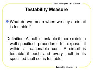
Testability Measure. What do we mean when we say a circuit is testable? Definition: A fault is testable if there exists a well-specified procedure to expose it within a reasonable cost. A circuit is testable if each and every fault in its specified fault set is testable. Keys To Testability.

E N D
Testability Measure What do we mean when we say a circuit is testable? Definition: A fault is testable if there exists a well-specified procedure to expose it within a reasonable cost. A circuit is testable if each and every fault in its specified fault set is testable.
Keys To Testability 1. Controllability 2. Observability 3. Predictability Testability = Controllability + Observability + Predictability
Design for Testability To constrain the design to make test generation and diagnosis easier.
Testability (Controllability/Observability) Measures 1. TMEAS [Stephenson & Grason, FTCS, 1976; DAC, 1979] 2. SCOAP [Goldstein, IEEE TCAS-26(9), 1979] 3. TESTSCREEN [Kovijanic 1979] 4. CAMELOT [Bennetts et al., 1980] 5. VICTOR [Ratiu et al., ITC, 1982]
Stephenson & Grason,s Approach Developed for register-transfer-level (RTL) circuits, but can also be applied at the gate level. The measures are normalized between 0 and 1 to reflect the ease of controlling and observing the internal nodes.
Stephenson & Grason,s Approach 1. For each signal line s, we denote the controllability of s as CY(s) and the observability of s as OY(s). 2. The values for the CYs and the OYs of all the signal lines are derived by solving a system of simultaneous equations with the CYs and the OYs as unknowns. The expression used to calculate CY for each output zj is where CTF is the controllability transfer factor of the component.
Stephenson & Grason,s Approach Let Nj(0) and Nj(1) be the numbers of input combinations for which zjhas value 0 and 1, respectively. Then 0 CTF 1. Each output controllability is assigned the same value.
Stephenson & Grason,s Approach The expression used to calculate OY for each input xi is where OTF is the observability transfer factor of the component.
Stephenson & Grason,s Approach Let NSibe the numbers of input combinations for which the change of xi results in a change of output. Then NSialso means the number of input combinations that can sensitize a path from xi to the output. The OTF measures the probability that a faulty value at any input will propagate to the outputs. 0 OTF 1 Each input observability is assigned the same value.
Stephenson & Grason,s Approach 3. Fanouts: Let s be a fanout stem and k be the number of its branches. Then the CYs of each fanout branch is The observability of the fanout stem s is where bi are fanout branches of s. 4. Sequential components: Sequential components are modeled by adding feedback links around the components that represent internal states .
Goldstein,s Approach---SCOAP Sandia Controllability Observability Analysis Program. The measures reflect the difficulty of controlling and observing the internal nodes; higher numbers indicate more difficult to control or observe. The measures are, in a sense, minimum cost values for controlling and observing.
Goldstein,s Approach---SCOAP Combinational 1- and 0-controllabilities of Y = AND(A,B,C): CC1(Y) =CC1(A) + CC1(B) + CC1(C) + 1; CC0(Y) = min{CC0(A),CC0(B),CC0(C)} + 1. The result is incremented by 1 so that the number reflects (in part) the distance to the PIs. Working breadth-first from PIs toward POs, we calculate the CC of the output line of each logic cell as a function of the CCs of its input lines.
Goldstein,s Approach---SCOAP The sequential controllability provides an estimate of the number of time frames needed to provide a 0 or 1 at a particular node. For Y=XOR(A, B): CC0(Y) = min{CC0(A) +CC0(B), CC1(A) + CC1(B)} + 1 CC1(Y) = min{CC0(A) + CC1(B), CC1(A) + CC0(B)} + 1 SC0(Y) = min{SC0(A) + SC0(B), SC1(A) + SC1(B)} SC1(Y) = min{SC0(A) + SC1(B), SC1(A) + SC0(B)} When computing the sequential controllabilities through combinational circuits, the values are not incremented---no additional time frames needed.
Goldstein,s Approach---SCOAP When deriving equations for sequential circuits, SCs are incremented by 1, but CCs are not incremented. Positive edge-triggered DFF with active low reset: CC0(Q) = min{CC0(R), CC1(R) + CC0(D) + CC0(C) + CC1(C)} CC1(Q) = CC1(R) + CC1(D) + CC0(C) + CC1(C) SC0(Q) = min{SC0(R), SC1(R) + SC0(D) + SC0(C) + SC1(C)} + 1 SC1(Q) = SC1(R) + SC1(D) + SC0(C) + SC1(C) + 1
Goldstein,s Approach---SCOAP Observabilities: CO(P) = CO(N) + CC1(Q) + CC1(R) + 1 SO(P) = SO(N) + SC1(Q) + SC1(R) Positive edge-triggered DFF with active low reset: CO(R) = CO(Q) + CC1(Q) + CC0(R) SO(R) = SO(Q) + SC1(Q) + SC0(R) +1 To watch R, then have to watch Q and drive FF to ,1, and then reset it to ,0,.
Goldstein,s Approach---SCOAP May define testability as follows: T(l/o) = CC1(l) + CO(l) T(l/1) = CC0(l) + CO(l) Initial Condition Node PI PO IN CC0 CC1 SC0 SC1 CO SO 1 1 1 1 1 1 - - - - 0 0 8 8 8 8 8 8
CAMELOT Controllability: CY(output) = CTF(output) x f(CYs(inputs)); controllability transfer factor where N(0) and N(1) are the numbers of input combinations for which the output has value 0 and 1, respectively.
CAMELOT CTF(NOT) = 1; CTF(NAND2) = 1/2; CTF(NAND3) = 1/4; CTF(ORn) =1/2n-1 CTF(XORn) = 1.
CAMELOT Q+ = [(JQ + KQ)C + QC]PR + P = JQCPR + KQCPR + QCPR + P Minterms in the final expression is 40; 24 invalid states; 16 common terms in this set of invalid states and the set of minterms derived above. N(1) = 40 - 16 = 24, and N(0) = (26 - 24) - N(1) = 40 - 24 = 16. CTF = 1- (24-16)/40 = 0.8. By symmetry, the CTF for Q+ is also 0.8.
CAMELOT CY(output) = CTF(output) x f(CYs(input)), where
CAMELOT Observability OY(at output) = OTF x OY(at input) x g(CYs(supporting inputs)), Where OTF is the observability transfer factor of the component for the input concerned.
CAMELOT where N(SP:I-O) is the total number of distinct sensitive paths from I to O, and N(IP:I-O) is the total number of insensi- tive paths.
CAMELOT OTF(NOT) = 1; OTF(NAND2) = 1/2 for each input; OTF(NAND3) = 1/4 for each input (1 PDC & 3 NPDCs); OTF (XORn) = 1 for each input (0 NPDC).
CAMELOT Let OY(A-B) denote the observability of node A at node B, then OY(I-O) = OTF(I-O) x OY(I-I) x CY(av), where
CAMELOT Fanouts: For a reconvergent fanout, select the shortest I-O path which is to be sensitized (while others are blocked), which is more likely to result in a higher OY. For feedback paths, the strategy is similar to that for reconvergent fanouts with unequal path lengths (i.e., select the shortest path).
CAMELOT Testability TY(node) = CY(node) x OY(node).
CAMELOT CAMELOT() 1. input, check, and initialize circuit; 2. calculate nodal CY values from PIs to POs; 3. calculate nodal OY values from POs to PIs; 4. calculate nodal TY values; 5. calculate TY and interpret the results;
Importance of Testability Measures They can guide the designers to improve the testability of their circuits. Test generation algorithms using heuristics usually apply some kind of testability measures to their heuristic operations (e.g., in making search decisions), which greatly speed up the test generation process.
Bibliography (1) J. E. Stephenson and J. Grason, ,,A testability measure for register transfer level digital circuits,,, in Proc. Int. Symp. Fault tolerant Computing (FTCS), (Pittsburgh, PA), pp. 101-107, June 1976. (2) J. Grason, ,,TMEAS-a testability measurement program,,, in Proc. IEEE/ACM Design Automation Conf. (DAC) , vol. 26, no. 9, pp. 156-161, 1979. (3) L. H. Goldstein, ,,Controllability/observability analysis for digital circuits,,, IEEE Trans. Circuits and Systems, vol. 26, no. 9, pp. 685-693, Sept. 1979. (4) P. G. Kovijanic, ,,Testability analysis,,, in Proc. IEEE Semiconductor Test Conf., pp. 310-316, 1979. (5) P. G. Kovijanic, ,,Computer-aided testability analysis,,, in Proc. IEEE Autotestcon, pp. 292-294, 1979. (6) R. G. Bennetts, C. M. Maunder, and G. D. Robinson, ,,CAMELOT:a computer-aided measure for logic testability,,, IEE Proc. Pt. E, vol. 128, no. 5, pp. 177-189, 1981. (7) R. G. Bennetts, Design of Testable logic Circuits. Reading, MA: Addison-Wesley, 1984.
Bibliography (8) I. M. Ratiu, A. Sangiovanni-Vincentelli, and D. O. Pederson, ,,VICTOR: a fast VLSI testability analysis program,,, in Proc. Int. Test Conf. (ITC), (Philadelphia, PA), pp. 397-401, Nov. 1982. (9) W. C. Berg and R. C. Hess, ,,COMET : a testability analysis and design modification package,,, in Proc. Int. Test Conf. (ITC), (Philadelphia, PA), pp. 364-378, Nov. 1982.