Download
1 / 40
410 likes | 640 Views
Feature matching and tracking Class 5. Read Section 4.1 of course notes http://www.cs.unc.edu/~marc/tutorial/node49.html Read Shi and Tomasi’s paper on good features to track http://www.unc.edu/courses/2004fall/comp/290/089/papers/shi-tomasi-good-features-cvpr1994.pdf

E N D
Feature matching and trackingClass 5 Read Section 4.1 of course notes http://www.cs.unc.edu/~marc/tutorial/node49.html Read Shi and Tomasi’s paper on good features to track http://www.unc.edu/courses/2004fall/comp/290/089/papers/shi-tomasi-good-features-cvpr1994.pdf Read Lowe’s paper on SIFT features http://www.unc.edu/courses/2004fall/comp/290/089/papers/Lowe_ijcv03.pdf
Feature matching vs. tracking Image-to-image correspondences are key to passive triangulation-based 3D reconstruction Extract features independently and then match by comparing descriptors Extract features in first images and then try to find same feature back in next view What is a good feature?
Comparing image regions Compare intensities pixel-by-pixel I(x,y) I´(x,y) Dissimilarity measures • Sum of Square Differences
Comparing image regions Compare intensities pixel-by-pixel I(x,y) I´(x,y) Similarity measures Zero-mean Normalized Cross Correlation
Feature points • Required properties: • Well-defined (i.e. neigboring points should all be different) • Stable across views (i.e. same 3D point should be extracted as feature for neighboring viewpoints)
Feature point extraction Find points that differ as much as possible from all neighboring points homogeneous edge corner
Feature point extraction • Approximate SSD for small displacement Δ • Image difference, square difference for pixel • SSD for window
Feature point extraction homogeneous edge corner Find points for which the following is maximum i.e. maximize smallest eigenvalue of M
Harris corner detector • Use small local window: • Maximize „cornerness“: • Only use local maxima, subpixel accuracy through second order surface fitting • Select strongest features over whole image and over each tile (e.g. 1000/image, 2/tile)
Simple matching • for each corner in image 1 find the corner in image 2 that is most similar (using SSD or NCC) and vice-versa • Only compare geometrically compatible points • Keep mutual best matches What transformations does this work for?
3 3 2 2 4 4 1 5 1 5 Feature matching: example What transformations does this work for? What level of transformation do we need?
Wide baseline matching • Requirement to cope with larger variations between images • Translation, rotation, scaling • Foreshortening • Non-diffuse reflections • Illumination geometric transformations photometric changes
Invariant detectors Rotation invariant Scale invariant Affine invariant
Normalization (Or how to use affine invariant detectors for matching)
Wide-baseline matching example (Tuytelaars and Van Gool BMVC 2000)
Lowe’s SIFT features (Lowe, ICCV99) Recover features with position, orientation and scale
Position • Look for strong responses of DOG filter (Difference-Of-Gaussian) • Only consider local maxima
Scale • Look for strong responses of DOG filter (Difference-Of-Gaussian) over scale space • Only consider local maxima in both position and scale • Fit quadratic around maxima for subpixel
Orientation • Create histogram of local gradient directions computed at selected scale • Assign canonical orientation at peak of smoothed histogram • Each key specifies stable 2D coordinates (x, y, scale, orientation)
SIFT descriptor • Thresholded image gradients are sampled over 16x16 array of locations in scale space • Create array of orientation histograms • 8 orientations x 4x4 histogram array = 128 dimensions
Matas et al.’s maximally stable regions • Look for extremal regions http://cmp.felk.cvut.cz/~matas/papers/matas-bmvc02.pdf
Feature tracking • Identify features and track them over video • Small difference between frames • potential large difference overall • Standard approach: KLT (Kanade-Lukas-Tomasi)
Good features to track • Use same window in feature selection as for tracking itself • Compute motion assuming it is small Affine is also possible, but a bit harder (6x6 in stead of 2x2) differentiate:
Example Simple displacement is sufficient between consecutive frames, but not to compare to reference template
Good features to keep tracking Perform affine alignment between first and last frame Stop tracking features with too large errors
Live demo • OpenCV (try it out!) LKdemo
Optical flow • Brightness constancy assumption (small motion) • 1D example possibility for iterative refinement
Optical flow • Brightness constancy assumption (small motion) • 2D example the “aperture” problem (1 constraint) ? (2 unknowns) isophote I(t+1)=I isophote I(t)=I
Optical flow • How to deal with aperture problem? (3 constraints if color gradients are different) Assume neighbors have same displacement
Lucas-Kanade Assume neighbors have same displacement least-squares:
Revisiting the small motion assumption • Is this motion small enough? • Probably not—it’s much larger than one pixel (2nd order terms dominate) • How might we solve this problem? * From Khurram Hassan-Shafique CAP5415 Computer Vision 2003
Reduce the resolution! * From Khurram Hassan-Shafique CAP5415 Computer Vision 2003
u=1.25 pixels u=2.5 pixels u=5 pixels u=10 pixels image It-1 image It-1 image I image I Gaussian pyramid of image It-1 Gaussian pyramid of image I Coarse-to-fine optical flow estimation slides from Bradsky and Thrun
warp & upsample run iterative L-K . . . image J image It-1 image I image I Gaussian pyramid of image It-1 Gaussian pyramid of image I Coarse-to-fine optical flow estimation slides from Bradsky and Thrun run iterative L-K
L2 M m2 C2 Next class: triangulation and reconstruction m1 C1 L1 Triangulation • calibration • correspondences