Download
1 / 33
350 likes | 739 Views
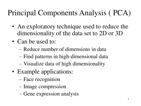
Principal Components Analysis. Objectives: Understand the principles of principal components analysis (PCA) Recognize conditions under which PCA may be useful Use SAS procedure PRINCOMP to perform a principal components analysis interpret PRINCOMP output. Typical Form of Data.

E N D
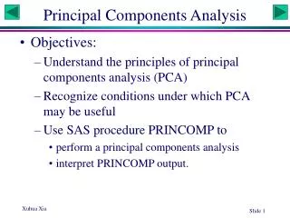
Principal Components Analysis • Objectives: • Understand the principles of principal components analysis (PCA) • Recognize conditions under which PCA may be useful • Use SAS procedure PRINCOMP to • perform a principal components analysis • interpret PRINCOMP output.
Typical Form of Data A data set in a 8x3 matrix. The rows could be species and columns sampling sites. 100 97 99 96 90 90 80 75 60 75 85 95 62 40 28 77 80 78 92 91 80 75 85 100 X = A matrix is often referred to as a nxp matrix (n for number of rows and p for number of columns). Our matrix has 8 rows and 3 columns, and is an 8x3 matrix. A variance-covariance matrix has n = p, and is called n-dimensional square matrix.
What are Principal Components? • Principal components are linear combinations of the observed variables. The coefficients of these principal components are chosen to meet three criteria • What are the three criteria? Y = b1X1 + b2 X2 + … bn Xn
What are Principal Components? • The three criteria: • There are exactly p principal components (PCs), each being a linear combination of the observed variables; • The PCs are mutually orthogonal (i.e., perpendicular and uncorrelated); • The components are extracted in order of decreasing variance.
A Simple Data Set X Y X 1 1 Y 1 1 X Y X 1 1.414 Y 1.414 2 Correlation matrix Covariance matrix
General Patterns • The total variance is 3 (= 1 + 2) • The two variables, X and Y, are perfectly correlated, with all points fall on the regression line. • The spatial relationship among the 5 points can therefore be represented by a single dimension. • PCA is a dimension-reduction technique. What would happen if we apply PCA to the data?
Graphic PCA 2 1.5 1 0.5 0 Y -0.5 -1 -1.5 -2 -1.5 -1 -0.5 0 0.5 1 1.5 X
SAS Program data pca; input x y; cards; -1.264911064 -1.788854382 -0.632455532 -0.894427191 0 0 0.632455532 0.894427191 1.264911064 1.788854382 ; proc princomp cov out=pcscore; proc print; var prin1 prin2; proc princomp data=pca out=pcscore; proc print; var prin1 prin2; run; Requesting the PCA to be carried out on the covariance matrix rather than the correlation matrix. Without specifying the covariance option, PCA will be carried out on the correlation matrix.
A positive definite matrix • When you run the SAS program, the log file will warn that “The Correlation Matrix is not positive definite.”. What does that mean? • A symmetric matrix M (such as a correlation matrix or a covariance matrix) is positive definite if z’Mz > 0 for all non-zero vectors z with real entries, where z’ is the transpose of z. • Given our correlation matrix with all entries being 1, it is easy to find z that lead to z’Mz = 0. So the matrix is not positive definite: Replace the correlation matrix with the covariance matrix and solve for z.
SAS Output Eigenvalues of the Covariance Matrix Eigenvalue Difference Proportion Cumulative PRIN1 3.00000 3.00000 1.00000 1.00000 PRIN2 0.00000 . 0.00000 1.00000 Eigenvectors PRIN1 PRIN2 X 0.577350 0.816497 Y 0.816497 -.577350 OBS PRIN1 PRIN2 1 -2.19089 0 2 -1.09545 0 3 0.00000 0 4 1.09545 0 5 2.19089 0 PC1 = 0.57735*X1+0.816497*X2 Variance accounted for by each principal components Principal component scores What’s the variance in PC1? How are the values computed?
SAS Output OBS PRIN1 PRIN2 1 -2.19089 0 2 -1.09545 0 3 0.00000 0 4 1.09545 0 5 2.19089 0
SAS Output Eigenvalues of the Correlation Matrix Eigenvalue Difference Proportion Cumulative PRIN1 2.00000 2.00000 1.00000 1.00000 PRIN2 0.00000 . 0.00000 1.00000 Eigenvectors PRIN1 PRIN2 X 0.707107 0.70710 Y 0.707107 -0.70711 OBS PRIN1 PRIN2 1 -1.78885 0 2 -0.89443 0 3 0.00000 0 4 0.89443 0 5 1.78885 0 Variance accounted for by each principal components Principal component scores What’s the variance in PC1?
Steps in a PCA • Have at least two variables • Generate a correlation or variance-covariance matrix • Obtain eigenvalues and eigenvectors (This is called an eigenvalue problem, and will be illustrated with a simple numerical example) • Generate principal component (PC) scores • Plot the PC scores in the space with reduced dimensions • All these can be automated by using SAS.
Covariance or Correlation Matrix? 40 30 Sp1 Abundance 20 Sp2 10 0
The Eigenvalue Problem The covariance matrix. The Eigenvalue is the set of values that satisfy this condition. The resulting eigenvalues (There are n eigenvalues for n variables). The sum of eigenvalues is equal to the sum of variances in the covariance matrix. Finding the eigenvalues and eigenvectors is called an eigenvalue problem (or a characteristic value problem).
Get the Eigenvectors • An eigenvector is a vector (x) that satisfies the following condition:A x = x • In our case A is a variance-covariance matrix of the order of 2, and a vector x is a vector specified by x1 and x2.
Get the Eigenvectors • We want to find an eigenvector of unit length, i.e., x12 + x22 = 1 • We therefore have From Previous Slide Solve x1 The first eigenvector is one associated with the largest eigenvalue.
Get the PC Scores First PC score Original data (x and y) Eigenvectors Second PC score The original data in a two dimensional space is reduced to one dimension..
What Are Principal Components? • Principal components are a new set of variables, which are linear combinations of the observed ones, with these properties: • Because of the decreasing variance property, much of the variance (information in the original set of p variables) tends to be concentrated in the first few PCs. This implies that we can drop the last few PCs without losing much information. PCA is therefore considered as a dimension-reduction technique. • Because PCs are orthogonal, they can be used instead of the original variables in situations where having orthogonal variables is desirable (e.g., regression).
Index of hidden variables • The ranking of Asian universities by the Asian Week • HKU is ranked second in financial resources, but seventh in academic research • How did HKU get ranked third? • Is there a more objective way of ranking? • An illustrative example:
A Simple Data Set • School 5 is clearly the best school • School 1 is clearly the worst school
Graphic PCA -1.7889 -0.8944 0 0.8944 1.7889
Crime Data in 50 States STATE MURDER RAPE ROBBE ASSAU BURGLA LARCEN AUTO ALABAMA 14.2 25.2 96.8 278.3 1135.5 1881.9 280.7 ALASKA 10.8 51.6 96.8 284.0 1331.7 3369.8 753.3 ARIZONA 9.5 34.2 138.2 312.3 2346.1 4467.4 439.5 ARKANSAS 8.8 27.6 83.2 203.4 972.6 1862.1 183.4 CALIFORNIA 11.5 49.4 287.0 358.0 2139.4 3499.8 663.5 COLORADO 6.3 42.0 170.7 292.9 1935.2 3903.2 477.1 CONNECTICUT 4.2 16.8 129.5 131.8 1346.0 2620.7 593.2 DELAWARE 6.0 24.9 157.0 194.2 1682.6 3678.4 467.0 FLORIDA 10.2 39.6 187.9 449.1 1859.9 3840.5 351.4 GEORGIA 11.7 31.1 140.5 256.5 1351.1 2170.2 297.9 HAWAII 7.2 25.5 128.0 64.1 1911.5 3920.4 489.4 IDAHO 5.5 19.4 39.6 172.5 1050.8 2599.6 237.6 ILLINOIS 9.9 21.8 211.3 209.0 1085.0 2828.5 528.6 . . . . . . . . . . . . . . . . PROC PRINCOMP OUT=CRIMCOMP;
DATA CRIME; TITLE 'CRIME RATES PER 100,000 POP BY STATE'; INPUT STATENAME $1-15 MURDER RAPE ROBBERY ASSAULT BURGLARY LARCENY AUTO; CARDS; Alabama 14.2 25.2 96.8 278.3 1135.5 1881.9 280.7 Alaska 10.8 51.6 96.8 284.0 1331.7 3369.8 753.3 Arizona 9.5 34.2 138.2 312.3 2346.1 4467.4 439.5 Arkansas 8.8 27.6 83.2 203.4 972.6 1862.1 183.4 California 11.5 49.4 287.0 358.0 2139.4 3499.8 663.5 Colorado 6.3 42.0 170.7 292.9 1935.2 3903.2 477.1 Connecticut 4.2 16.8 129.5 131.8 1346.0 2620.7 593.2 Delaware 6.0 24.9 157.0 194.2 1682.6 3678.4 467.0 Florida 10.2 39.6 187.9 449.1 1859.9 3840.5 351.4 Georgia 11.7 31.1 140.5 256.5 1351.1 2170.2 297.9 Hawaii 7.2 25.5 128.0 64.1 1911.5 3920.4 489.4 Idaho 5.5 19.4 39.6 172.5 1050.8 2599.6 237.6 Illinois 9.9 21.8 211.3 209.0 1085.0 2828.5 528.6 Indiana 7.4 26.5 123.2 153.5 1086.2 2498.7 377.4 Iowa 2.3 10.6 41.2 89.8 812.5 2685.1 219.9 Kansas 6.6 22.0 100.7 180.5 1270.4 2739.3 244.3 Kentucky 10.1 19.1 81.1 123.3 872.2 1662.1 245.4 Louisiana 15.5 30.9 142.9 335.5 1165.5 2469.9 337.7 Maine 2.4 13.5 38.7 170.0 1253.1 2350.7 246.9 Maryland 8.0 34.8 292.1 358.9 1400.0 3177.7 428.5 Massachusetts 3.1 20.8 169.1 231.6 1532.2 2311.3 1140.1 Michigan 9.3 38.9 261.9 274.6 1522.7 3159.0 545.5 Minnesota 2.7 19.5 85.9 85.8 1134.7 2559.3 343.1 Mississippi 14.3 19.6 65.7 189.1 915.6 1239.9 144.4 Missouri 9.6 28.3 189.0 233.5 1318.3 2424.2 378.4 Montana 5.4 16.7 39.2 156.8 804.9 2773.2 309.2 Nebraska 3.9 18.1 64.7 112.7 760.0 2316.1 249.1 Nevada 15.8 49.1 323.1 355.0 2453.1 4212.6 559.2 New Hampshire 3.2 10.7 23.2 76.0 1041.7 2343.9 293.4 New Jersey 5.6 21.0 180.4 185.1 1435.8 2774.5 511.5 New Mexico 8.8 39.1 109.6 343.4 1418.7 3008.6 259.5 New York 10.7 29.4 472.6 319.1 1728.0 2782.0 745.8
North Carolina 10.6 17.0 61.3 318.3 1154.1 2037.8 192.1 North Dakota 0.9 9.0 13.3 43.8 446.1 1843.0 144.7 Ohio 7.8 27.3 190.5 181.1 1216.0 2696.8 400.4 Oklahoma 8.6 29.2 73.8 205.0 1288.2 2228.1 326.8 Oregon 4.9 39.9 124.1 286.9 1636.4 3506.1 388.9 Pennsylvania 5.6 19.0 130.3 128.0 877.5 1624.1 333.2 Rhode Island 3.6 10.5 86.5 201.0 1489.5 2844.1 791.4 South Carolina 11.9 33.0 105.9 485.3 1613.6 2342.4 245.1 South Dakota 2.0 13.5 17.9 155.7 570.5 1704.4 147.5 Tennessee 10.1 29.7 145.8 203.9 1259.7 1776.5 314.0 Texas 13.3 33.8 152.4 208.2 1603.1 2988.7 397.6 Utah 3.5 20.3 68.8 147.3 1171.6 3004.6 334.5 Vermont 1.4 15.9 30.8 101.2 1348.2 2201.0 265.2 Virginia 9.0 23.3 92.1 165.7 986.2 2521.2 226.7 Washington 4.3 39.6 106.2 224.8 1605.6 3386.9 360.3 West Virginia 6.0 13.2 42.2 90.9 597.4 1341.7 163.3 Wisconsin 2.8 12.9 52.2 63.7 846.9 2614.2 220.7 Wyoming 5.4 21.9 39.7 173.9 811.6 2772.2 282.0 ; PROCPRINCOMP out=crimcomp; run; PROCPRINT; ID STATENAME; VAR PRIN1 PRIN2 MURDER RAPE ROBBERY ASSAULT BURGLARY LARCENY AUTO; run; PROCGPLOT; PLOT PRIN2*PRIN1=STATENAME; TITLE2 'PLOT OF THE FIRST TWO PRINCIPAL COMPONENTS'; run; PROCPRINCOMP data=CRIME COV OUT=crimcomp; run; PROCPRINT; ID STATENAME; VAR PRIN1 PRIN2 MURDER RAPE ROBBERY ASSAULT BURGLARY LARCENY AUTO; run; /* Add to have a map view*/ procsort data=crimcomp out=crimcomp; by STATENAME; run; procsort data=maps.us2 out=mymap; by STATENAME; run; data both; merge mymap crimcomp; by STATENAME; run; procgmap data=both; id _map_geometry_; choro PRIN1 PRIN2/levels=15; /* choro PRIN1/discrete; */ run;
Correlation Matrix MURDER RAPE ROBBERY ASSAULT BURGLARY LARCENY AUTO MURDER 1.0000 0.6012 0.4837 0.6486 0.3858 0.1019 0.0688 RAPE 0.6012 1.0000 0.5919 0.7403 0.7121 0.6140 0.3489 ROBBERY 0.4837 0.5919 1.0000 0.5571 0.6372 0.4467 0.5907 ASSAULT 0.6486 0.7403 0.5571 1.0000 0.6229 0.4044 0.2758 BURGLARY 0.3858 0.7121 0.6372 0.6229 1.0000 0.7921 0.5580 LARCENY 0.1019 0.6140 0.4467 0.4044 0.7921 1.0000 0.4442 AUTO 0.0688 0.3489 0.5907 0.2758 0.5580 0.4442 1.0000 If variables are not correlated, there would be no point in doing PCA. The correlation matrix is symmetric, so we only need to inspect either the upper or lower triangular matrix.
Eigenvalues Eigenvalue Difference Proportion Cumulative PRIN1 4.11496 2.87624 0.587851 0.58785 PRIN2 1.23872 0.51291 0.176960 0.76481 PRIN3 0.72582 0.40938 0.103688 0.86850 PRIN4 0.31643 0.05846 0.045205 0.91370 PRIN5 0.25797 0.03593 0.036853 0.95056 PRIN6 0.22204 0.09798 0.031720 0.98228 PRIN7 0.12406 . 0.017722 1.00000
Eigenvectors • Do these eigenvectors mean anything? • All crimes are positively correlated with the first eigenvector, which is therefore interpreted as a measure of overall crime rate. • The 2nd eigenvector has positive loadings on AUTO, LARCENY and ROBBERY and negative loadings on MURDER, ASSAULT and RAPE. It is interpreted to measure the preponderance of property crime over violent crime…... PRIN1 PRIN2 PRIN3 PRIN4 PRIN5 PRIN6 PRIN7 MURDER 0.3002 -.6291 0.1782 -.2321 0.5381 0.2591 0.2675 RAPE 0.4317 -.1694 -.2441 0.0622 0.1884 -.7732 -.2964 ROBBERY 0.3968 0.0422 0.4958 -.5579 -.5199 -.1143 -.0039 ASSAULT 0.3966 -.3435 -.0695 0.6298 -.5066 0.1723 0.1917 BURGLARY 0.4401 0.2033 -.2098 -.0575 0.1010 0.5359 -.6481 LARCENY 0.3573 0.4023 -.5392 -.2348 0.0300 0.0394 0.6016 AUTO 0.2951 0.5024 0.5683 0.4192 0.3697 -.0572 0.1470
PC Plot: Crime Data Maryland Nevada, New York, California North and South Dakota Mississippi, Alabama, Louisiana, South Carolina