Download
1 / 29
290 likes | 479 Views
Big Bang, Big Iron High Performance Computing and the Cosmic Microwave Background. Julian Borrill Computational Cosmology Center, LBL Space Sciences Laboratory, UCB and the BOOMERanG , MAXIMA, Planck, EBEX & PolarBear collaborations. The Cosmic Microwave Background.

E N D
Big Bang, Big IronHigh Performance Computing and the Cosmic Microwave Background Julian Borrill Computational Cosmology Center, LBL Space Sciences Laboratory, UCB and the BOOMERanG, MAXIMA, Planck, EBEX & PolarBear collaborations
The Cosmic Microwave Background About 400,000 years after the Big Bang, the expanding Universe cools through the ionization temperature of hydrogen: p+ + e- => H. Without free electrons to scatter off, the photons free-stream to us today. • COSMIC - filling all of space. • MICROWAVE - redshifted by the expansion of the Universe from 3000K to 3K. • BACKGROUND - primordial photons coming from “behind” all astrophysical sources.
CMB Science • Primordial photons give the earliest possible image of the Universe. • The existence of the CMB supports a Big Bang over a Steady State cosmology (NP1). • Tiny fluctuations in the CMB temperature (NP2) and polarization encode the fundamentals of • Cosmology • geometry, topology, composition, history, … • Highest energy physics • grand unified theories, the dark sector, inflation, … • Current goals: • definitive T measurement provides complementary constraints for all dark energy experiments. • detection of cosmological B-mode gives energy scale of inflation from primordial gravity waves. (NP3)
The Concordance Cosmology Supernova Cosmology Project (1998): Cosmic Dynamics (- m) BOOMERanG & MAXIMA (2000): Cosmic Geometry (+ m) 70% Dark Energy + 25% Dark Matter + 5% Baryons 95% Ignorance What (and why) is the Dark Universe ?
Observing the CMB • With very sensitive, very cold, detectors. • Scanning all of the sky from space, or just some of it from the stratosphere or high dry ground.
CMB Satellite Evolution Evolving science goals require (i) higher resolution & (ii) polarization sensitivity.
CMB Data Analysis • In principle very simple • Assume Guassianity and maximize the likelihood • of maps given theobservationsandtheirnoise statistics (analytic). • of power spectra given maps and their noise statistics (iterative). • In practice very complex • Foregrounds, glitches, asymmetric beams, non-Gaussian noise, etc. • Algorithm & implementation scaling with evolution of • CMB data-set size • HPC architecture
The CMB Data Challenge • Extracting fainter signals (polarization, high resolution) from the data requires: • larger data volumes to provide higher signal-to-noise. • more complex analyses to control fainter systematic effects. • 1000x increase in data volume over next 15 years • need linear analysis algorithms to scale through next 10 M-foldings!
CMB Data Analysis Evolution Data volume & computational capability dictate analysis approach.
Scaling In Practice • 2000: BOOMERanG T-map • 108 samples => 105 pixels • 128 Cray T3E processors; • 2005: Planck T-map • 1010 samples => 108pixels • 6000 IBM SP3 processors; • 2008: EBEX T/P-maps • 1011 samples, 106pixels • 15360 Cray XT4 cores. • 2010: Planck Monte Carlo 1000 noise T-maps • 1014 samples => 1011 pixels • 32000 Cray XT4 cores.
Planck Sim/Map Target • For Planck to publish its results in time, by mid-2012 we need to be able to simulate and map • O(104) realizations of the entire mission • 74 detectors x 2.5 years ~ O(1016) samples • On O(105) cores • In O(10) wall-clock hours WAIT ~ 1 day : COST ~ 106 CPU-hrs
TARGET: 104 maps 9 freqs 2.5 years 105 cores 10 hours CTP3 FFP1 M3/GCP OTFS Hybrid/ Peta-Scaling 12x217
Simulation & Mapping: Calculations Given the instrument noise statistics & beams, a scanning strategy, and a sky: • SIMULATION: dt = nt + st= nt + Ptp sp • A realization of the piecewise stationary noise time-stream: • Pseudo-random number generation & FFT • A signal time-stream scanned & beam-smoothed from the sky map: • SHT • MAPPING: (PT N-1 P) dp = PT N-1dt(A x = b) • Build the RHS • FFT & sparse matrix-vector multiply • Solve for the map • PCG over FFT & sparse matrix-vector multiply
Simulation & Mapping: Scaling • In theory such analyses should scale • Linearly with the number of observations. • Perfectly to arbitrary numbers of cores. • In practice this does not happen because of • IO (reading pointing; writing time-streams reading pointing & timestreams; writing maps) • Communication (gathering maps from all processes) • Calculation inefficiency (linear operations only) • Code development has been an ongoing history of addressing these challenges anew with each new data volume and system concurrency.
IO - Before For each MC realization For each detector Read detector pointing Sim Write detector timestream For all detectors Read detector timestream & pointing Map Write map • Read: 56 x Realizations x Detectors x Observations bytes Write: 8 x Realizations x (Detectors x Observations + Pixels) bytes E.g. for Planck, read 500PB & write 70PB.
IO - Optimizations • Read sparse telescope pointing instead of dense detector pointing • Calculate individual detector pointing on the fly. • Remove redundant write/read of time-streams between simulation & mapping • Generate simulations on the fly only when map-maker requests data. • Put MC loop inside map-maker • Amortize common data reads over all realizations.
IO – After Now Read telescope pointing For each detector Calculate detector pointing For each MC realization SimMap For all detectors Simulate time-stream Write map • Read: 24 x Sparse Observations bytes Write: 8 x Realizations x Pixels bytes E.g. for Planck, read 2GB & write 70TB (108 read & 103 write compression).
Communication Details • The time-ordered data from all the detectors are distributed over the processes subject to: • Load-balance • Common telescope pointing • Each process therefore holds • some of the observations • for some of the pixels. • In each PCG iteration, each process solves with its observations. • At the end of each iteration, each process needs to gather the total result for all of the pixels in its subset of the observations.
Communication - Before • Initialize a process & MPI task on every core • Distribute time-stream data & hence pixels • After each PCG iteration • Each process creates a full map vector by zero-padding • Call MPI_Allreduce(map, world) • Each process extracts the pixels of interest to it & discards the rest
Communication – Optimizations • Reduce the number of MPI tasks • Use threads for on-node communication • Only use MPI for off-node communication • Minimize the total volume of the messages • Determine processes’ pair-wise pixel overlap • If the data volume is smaller, use gathers in place of reduces
Communication – After Now • Initialize a process & MPI task on every node • Distribute time-stream data & hence pixels • Calculate common pixels for every pair of processes • After each PCG iteration • If most pixels are common to most processes • use MPI_Allreduce(map, world) as before • Else • Each process prepares its send buffer • Call MPI_Alltoallv(sbuffer, rbuffer, world) • Each process receives contributions only to the pixels of interest to it & sums them.
Communication - Impact Fewer communicators & smaller message volume:
HPC System Evaluation • Well-characterized & -instrumented science application codes can be a powerful tool for whole-system performance evaluation. • Compare • unthreaded/threaded • allreduce/allgather on Cray XT4, XT5, XE6 on 200 – 16000 cores
Current Status • Calculation scale with #observations. • IO & communication scale with #pixels. • Observations/pixel ~ S/N: science goals will help scaling! • Planck: O(103) observations per pixel • PolarBear: O(106) observations per pixel • For each experiment, fixed data volume => strong scaling. • Between experiments, growing data volume => weak scaling.
HPC System Evolution • Clock speed is no longer able to maintain Moore’s Law. • Multi-core CPU and GPGPU are two major approaches. • Both of these will require • significant code development • performance experiments & auto-tuning • E.g. NERSC’s new XE6 system Hopper • 6384 nodes • 2 sockets per node • 2 NUMA nodes per socket • 6 cores per NUMA node • What is the best way to run hybrid code on such a system?
Conclusions • The CMB provides a unique window onto the early Universe • investigate fundamental cosmology & physics. • The CMB data sets we gather and the HPC systems we analyze them on are both evolving. • CMB data analysis is a long-term computationally-challenging problem requiring state-of-the-art HPC capabilities. • The science we can extract from present and future CMB data sets will be determined by the limits on • our computational capability, and • our ability to exploit it.