Download
1 / 18
190 likes | 359 Views
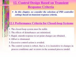
12. Control Design Based on Transient Response Criteria. In this chapter, we consider the selection of PID controller settings based on transient response criteria. 12.1 Performance Criteria for Closed-loop Systems. 1. The closed-loop system must be stable.

E N D
12. Control Design Based on Transient Response Criteria • In this chapter, we consider the selection of PID controller settings based on transient response criteria. 12.1 Performance Criteria for Closed-loop Systems 1. The closed-loop system must be stable. 2. The effects of disturbances are minimized. 3. Rapid, smooth response to set-point changes are obtained. 4. Offset is eliminated. 5. Excessive control action is avoided. 6. The control system is robust, that is, it is insensitive to changes in process conditions and to errors in the assumed process model.
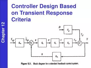
12.2 Direct Synthesis Method • A feedback controller can be designed by using a process model and specifying the desired closed-loop response. Advantage : it provides insight about the relation between the process and the resulting controller. Disadvantage : the resulting controllers may not have a PID structure. Figure 12.1. Block diagram for a standard feedback control system
If the unknown G is replaced by an assumed process model and if C/R is replaced by a desired closed-loop transfer function (C/R)d ; The closed-loop transfer function for set-point change. For simplicity, let G = GvGpGm , Gm = Km. Then, (12.1) reduces Rearranging gives an expression for the feedback controller. For ideal case
These equations indicate that for the product GcG, controller poles cancel process zeros while the controller zeros cancel the process poles. • Since these pole-zero cancellations are seldom exact sue to modeling errors, the Direct Synthesis approach should be used with caution for processes that have unstable poles or zeros. 12.2.1 Perfect Control When the controlled variable tracks set-point changes instantaneously without any error, this situation is referred to as perfect control. Thus, (C/R)d = 1 or C = R. ⇒ impossible since the required controller in Eq.(12.3) would require an infinite gain.
12.2.2 Controllers Designed to Give Finite Settling Times The controller considered in the previous section are unrealistic since the design objective was to have the process reach a new set point instantaneously. A more practical approach is to specify C/R so that realistic setting times are achieved. For example, suppose that the desired closed-loop transfer function is (C/R)d = 1/(tcs + 1). • the desired closed-loop response to a step change in set-point would response as a first-order process with time constant tc . Note) 1/tcsterm provides I-control action (zero offset).
12.2.3 Process with Time Delays where qc and tc are design parameters (qcq ;q is process time delay). Combining Eq. (12.4) and Eq. (12.3) and let qc =q gives, this controller does not have the standard PID form but is physically realizable. Approximating the time-delay term in the denominator by a first-order Taylor series expansion; exp(-qcs) 1-qs
Note) in this approach it is not necessary to approximate the time-delay term in the numerator because it is canceled by the identical term in G(s). Next we consider two special cases Case a. First-Order plus Time-Delay Model Substituting Eq. (12.6) into Eq. (12.5) where, • Kc should be reduced when the process contains a time delay.
Case b. Second-Order plus Time-Delay Model Substituting Eq. (12.8) into Eq. (12.5) where, • PI and PID controller in Eqs. (12.7) and (12.9) provide approximate time delay compensation. • Controller settings obtained from the Direct Synthesis method can be made more conservative by increasing tc . • A conservative choice of tc is prudent when q /t is significant, since the controller design equations, Eqs. (12.7) and (12.9), were derived based on set-point responses and first-order approximations for the time delay term.
12.3 Internal Model Control • based on an assumed process model and relates the controller settings to the model parameters in a straightforward manner. Advantage : 1. It explicitly takes into account model uncertainty. 2. It allows the designer to trade-off control system performance against control system robustness to process changes and modeling errors. Figure 12.2. Feedback control Strategies
The two block diagrams are identical if controllers Gc and satisfy the relation For the special case of a perfect model (G = ), Eq.(12.11) reduces to The following closed-loop relation for IMC can be derived from Fig. 12.2b:
where contains any time delays and right-half plane zeros. is specified so that its steady-state gain is one. The IMC controller is designed in two steps. Step 1. The process model is factored as Step 2. The controller is specified as where f is a low-pass filter with a steady-state gain of one. The IMC filter f typically has the form.
where tc is the desired closed-loop time constant. Parameter r is a positive integer that is selected so that is either a proper transfer function. Note) • The IMC controller in Eq.(12.14) includes the inverse of rather than the inverse of the entire process model . • In contrast, if had been used, the controller would contain a prediction term eqs(if contained a time delay q) or an unstable pole (if contained a right-half plane zero). • Thus, by employing the factorization given in (12.13) and using a filter of the form of (12.15), the resulting controller is guaranteed to be physically realizable and stable. • Since the IMC controller in (12.14) is based on pole-zero cancellation, the IMC approach should not be used for processes that are open-loop unstable.
Table 12.1. IMC-Based PID Controller Settings for Gc(s) Although the process models in Table 12.1 do not explicitly contain time delays, such models can be accommodated by introducing Padé approximations or power series expansions for the time delay terms.
12.4 Design Relations for PID Controllers • In this section we consider some well-known controller design relations that are based on a specific model, namely the FOPTD model. • Cohen and Coon method Empirical design relation to provide closed-responses with a decay ratio 1/4 ⇒ needed process information ( FOPTD model) ⇒ determined from experimental step response data. Table 12.2.Cohen and Coon Controller Design Relations
only gives initial setting since determined from first two peaks. - Disadvantages (performance criterion) 1. Responses with 1/4 decay ratios are often judged to be too oscillatory by plant operating personnel. 2. The criterion considers only two points of the closed-loop response c(t), namely the first two peaks.
12.4.1 Design Relations based on Integral Error Criteria Three popular performance indices. 1. Integral of the absolute value of the error (IAE) where the error signal e(t) is the difference between the set point and the measurement. 2. Integral of the squared error (ISE) 3. Integral of the time-weighted absolute error (ITAE) • The ISE criterion tends to place a greater penalty on large errors than the IAE or ITAE criteria. • The ITAE criterion penalizes errors that persist for long periods of time. • In general, ITAE is the preferred integral error criterion since it results in the most conservative controller settings.
Lopez et al. (1967) obtained the optimal tuning parameters by solving (12.18) for various FOPTD model and then fitted the obtained optimal data sets as follows. Table 12.3.Controller Design Relations based on the ITAE Performance Index and a FOPTD Model.
12.5 Comparison of Controller Design Relations 1. Kc 1/K where K = KvKpKm . 2. q /t ↑ Kc ↓ (more time delay → poorer performance) 3. q /t ↑ tI and tD ↑ ( tD / tI = 0.1 ∼ 0.3 ) 4. When integral control action is added to a proportional-only controller, Kc ↓ the addition of derivative action Kc ↑ (stability margin increased) 5. The Cohen-Coon design relations tend to yield oscillatory closed-loop responses since the design objective is a 1/4 decay ratio. If less oscillatory responses are desired, Kc ↓ and tI ↑. 6. ITAE → most conservative settings ISE → least conservative settings.