Download
1 / 42
420 likes | 490 Views
Instrumentation Concepts Ground-based Optical Telescopes. Keith Taylor (IAG/USP) Aug-Nov, 2008. IAG-USP (Keith Taylor). Aug-Sep, 2008. and Signal to Noise Ratios. CCDs in Astronomy.

E N D
IAG/USP (Keith Taylor) Instrumentation ConceptsGround-based Optical Telescopes Keith Taylor (IAG/USP) Aug-Nov, 2008 IAG-USP (Keith Taylor) Aug-Sep, 2008
and Signal to Noise Ratios CCDs in Astronomy Charged coupled devices (CCD's) have been used in astronomy since the late 1970's. They are now nearly ubiquitous in observations made at wavelengths between the near-IR (~1µm) and the X-ray. They have transformed the way astronomy is done. IAG/USP (Keith Taylor)
IAG/USP (Keith Taylor) GENERAL DETECTOR CHARACTERIZATION(Quantum Efficiency = QE) • QE = percentage of photons incident on detector which produce measurable signals • Strong wavelength dependence (e.g. threshold activation cutoffs set by workfunction/band gap) • Typical peak values: • Eye: 1-2% • Photographic plate: 1-2% • Photomultiplier tube: 20-30% • CCD: 70-90% • IR array (HgCdTe): 50-80% • Schematic QE curves for various classes of detector • "Detective quantum efficiency" = [(SNRout)/(SNRin)]2, where "in" and "out" refer to the input and output signals to/from the detector, respectively. DQE combines basic QE with the noise introduced by the detector. This quantity is really what matters in comparing detectors, but it is so dependent on specific details of operations/applications that it is rarely used. • SPECTRAL RANGE • Wavelength region over which QE is sufficient for operation
IAG/USP (Keith Taylor) Dynamic Range • Definition: ratio of maximum to minimum measurable signal • eg: maximum number of events in a single CCD pixel is determined by photoelectron "full well'' capacity or digitization maximum (typically 2 bytes); minimum is determined by dark current/readout noise • Applies to a single exposure; effective dynamic range can be increased with multiple exposures • Typical values: 102(Pg); 104 (CCD); 105 (PMT) • Related concepts: • Linear Range: range of signals for which [Output] = k x [Input], where k is a constant. Generally smaller than calibrateable range • Threshold: minimum measurable signal. Influenced by detector noise or other intrinsic characteristics (e.g. fog on Pg plates) • Saturation point: level where detector response ceases to change with signal
IAG/USP (Keith Taylor) FLUX MEASUREMENTSAND SIGNAL-TO-NOISE RATIOS Comparison of photographic and CCD exposures of same field with 4-m. 45 min photographic plate 2 hr CCD (stacked)
IAG/USP (Keith Taylor) Hale’s Lament “Starlight is falling on every square mile of the Earth’s surface, and the best we can do is gather up and concentrate the rays that strike an area 100 inches in diameter.” [G. E. Hale, 1928] In 75 years, we have progressed to 10m diameters for optical telescopes, but we still collect a pitifully small fraction of the photons incident from cosmic sources. What are the important considerations in making optimal use of the photons we do have at our disposal?
IAG/USP (Keith Taylor) The Observer’s Problem • The Problem: How to maximize the reliable astrophysical content of observations? • How to make accurate flux measurements with a precision or SNR appropriate to the scientific goals given the practical constraints?
IAG/USP (Keith Taylor) Key factors affecting SNR • Source: Luminosity and distance • Brightness is usually a strong function of wavelength • Destruction or deflection of source photons on way to detection • Noise in process of measuring source photons • Telescope size • Background photons • Bandwidth (should be maximum consistent with desired information content) • Instrument throughput, detector sensitivity, noise characteristics • “Detective quantum efficiency”= DQE = [SNRout/SNRin]2 • Extent to which equipment can be calibrated to characterize random and systematic errors. • Real-world time constraints on access to equipment & therefore exposure times
IAG/USP (Keith Taylor) Mechanisms for Photon Destruction/Deflection These effects are mostly not stochastic in character. They must be calibrated for good accuracy in the results; will produce systematic errors if this is not done properly. • Almost all become more important at shorter wavelengths • Interstellar extinction • Depends on dust grain column density in direction of source • Atmospheric extinction • Depends on total atmospheric path length ( sec(z), where “z” is the angular distance to the zenith) • Atmospheric refraction • Prismatic effect of differential refraction for z > 0 causes elongation/chromatic separation of point sources • Atmospheric turbulence (“seeing”) • Causes blurring and jitter of images • Absorption/scattering by optical surfaces • Reflecting and refracting surfaces and transmitting media destroy a large fraction of photons incident on the telescope aperture
IAG/USP (Keith Taylor) Statistical Models of Flux Measurements • Every EM flux measurement is affected by stochastic processes. • Every time you try to determine the SNR of a measurement, you are applying an implicit statistical model for the parent distribution. • The appropriate model will differ with the instrument, detector, and waveband. In principle, each system should be analyzed separately. Rules of thumb for one do not necessarily apply to others. • The discussion here is aimed at observations made with CCD detectors
IAG/USP (Keith Taylor) Gaussian Distributions? • We can assume that most stochastic components entering astronomical flux measurements are governed by a Gaussian parent distribution. • Photon noise, the fundamental source of EM noise, is governed by Poisson/Gaussian statistics in practice. • However, other aspects of photon detection (e.g. amplifier gain variations, seeing variations, dark current, atmospheric transparency changes, etc.) may not be Gaussian. For instance, airglow emission lines usually vary non-randomly. Other elements of a detection system might be governed by Lorentzian or log-normal distributions. For accurate work, it is important to empirically confirm the nature of the statistics governing your measurements. • The BEST approach to error estimation is always to make many repeated measures of a value, say N > 10. But in practice this may be difficult.
IAG/USP (Keith Taylor) Sources of Noise in UVOIR Flux Measures • The major contributors to noise in UVOIR flux measurements are: • Photon noise • Background noise • Measuring process noise • Other sources of noise
IAG/USP (Keith Taylor) Photon Noise • Fundamental statistical fluctuations in photon arrival times imply that the photon count rate is a random variable (even if the source is strictly constant in luminosity). • Photon arrivals from most astronomical sources are an independent counting process and are described by Poisson statistics (for small mean counts per unit time) or Gaussian statistics (for larger means). • Photon statistics apply both to source photons and background photons.
IAG/USP (Keith Taylor) Implications of photon statistics • If we consider only noise from photon counting statistics from the source of interest, then: • SNR = N/(N) = N/N½ = N½, where N is the total number of source photons counted. • Known as “root N statistics”: N SNR 100 10 1000 32 10000 100 • Because of the contribution of other sources of noise in real measurements, these values are upper limits to the combined SNR.
IAG/USP (Keith Taylor) Caveats on Photon Statistics • Photons are Bose-Einstein particles, which means that a given quantum state can contain many photons. This gives rise to photon “bunching”. • In a photon stream originating in TEQ, the variance in photon arrivals is larger than for a Poisson process: 2(n) = n(1 + ), where = 1/(eh/kT − 1) • The correction term is important if > 2/T cm — i.e. in the infrared for normal stellar temperatures. • However, because typical detection systems (optics, detectors) are inefficient, the probability that more than one bunched photon will be detected is small, and the bunching effect can usually be ignored in practice. Photon bunching could be more important in non-thermal sources. • Hanbury-Brown and Twiss (1958) built a special optical “intensity interferometer” which took advantage of the bunching effect to measure the diameters of a small number of hot, bright stars.
IAG/USP (Keith Taylor) Background Noise • Background light sources are affected by photon statistics but in some cases (e.g. Earth’s atmosphere) also by intrinsic variations in flux.
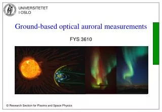
IAG/USP (Keith Taylor) Diffuse Sky Photon Background • Earth’s atmosphere: scattered city lights, airglow, aurorae, thermal continuum (IR). • Both continuum & emission lines. • Emission lines (e.g. [O I] and OH) can be highly variable. • Moonlight: drastic (> 3 mag arcsec−2) effect on brightness of optical sky background, depending on phase. Scattered moonlight is blue, so red/IR observations preferred when Moon is bright. • “Bright time”: Full Moon ±5 days • “Dark time”: New Moon ±5 days; reserved for faint target astronomy at most observatories. • Zodiacal light (sunlight scattered by Inter-Planetary grains); strong directional dependence, but not time dependence: • Has Solar spectrum + Thermal emission in IR. • Galactic background light. In UVOIR, is primarily starlight scattered by Inter-Stellar grains at lower galactic latitudes; has hot-star spectrum but is faint. • Mid, Far-IR ( > 20m) emission from warm dust: “IR cirrus”
IAG/USP (Keith Taylor) Broad-band (continuum & line emission)sky background levels (no Moon) at Mauna KeaNote dramatically increased brightness for JHK bands.
IAG/USP (Keith Taylor) Night sky spectrum from KPNO Shows red continuum, Hg, and Na emission lines from scattered city lights. (HPS = “high pressure sodium” lamps). Strong [O I] lines are auroral. Region redward of 6200Å shows start of forest of upper-atmospheric OH lines, which continues through near-IR.
IAG/USP (Keith Taylor) Night sky emission lines (mainly OH), near-IR Shows continuation of atmospheric OH spectrum from preceding KPNO plot. OH forms at 75 km altitude, so affects all ground-based sites. Impact of lines is devastating for certain kinds of observations. Natural extra-atmospheric background at these wavelengths is up to 1000 times fainter.
IAG/USP (Keith Taylor) Growth of city light contamination (A. Walker) No sites are free of serious & increasing light pollution except McDonald Observatory (in west Texas, where apparently nobody wants to live).
IAG/USP (Keith Taylor) Hemispheric images of far-infrared “cirrus” (COBE/DIRBE) “Cirrus” emission is produced by warm interstellar dust grains at typical distances of 100-3000 pc within the Galaxy. Far-IR (50–200μm) observations can be importantly affected by this strongly non-uniform background. Must make good determination of local 2D cirrus structure in order to remove its effects.
IAG/USP (Keith Taylor) BACKGROUND NOISE(Discrete Cosmic Sources) • Field stars (e.g. scattered light from bright stars; produce an “exclusion zone” around stars) • Star light scattered, refracted, or diffracted by the atmosphere and by telescope optics and structures can produce effects at large distances from a star. King (1971) showed that the profile of a star image has a Gaussian core, but then an exponential shoulder and a power law at r > 30 arcsec. • Extended envelopes from nearby galaxies • Faint distant galaxies (serious problem at faint levels since are thousands per square degree) • “Confusion” caused by source blending within spatial resolution cell. More serious in radio astronomy, but a major UVOIR problem in some cases, e.g. star clusters
IAG/USP (Keith Taylor) Detector Noise • “Dark current”: thermal emission in absence of signal; major problem; requires detector cooling • For a semiconductor such as a CCD array, the dark current behaves as: ndark = AT⅔e−Eg/2kT , where Eg is the band gap energy and T is the temperature. • Is a more serious problem for IR detectors because of smaller band gaps. • Cerenkov photons (cosmic rays) • CCDs: variations in electronic “bias”
IAG/USP (Keith Taylor) Telescope Backgrounds • IR: emission (T ~280 K) of optics and other structures visible to detector ( > 1.5m) • Diffraction & scattering (e.g. from dust on optics) contributes to background at all s. Note the ADVANTAGE of 2D digital array detectors for background determination: • Ordinarily 2D devices provide a large number of background samples surrounding a source of interest. The samples are also usually obtained (in imaging, for instance) simultaneously with the source observations, which is very important in the case of large & variable backgrounds. • As long as the background contains only low spatial frequencies, it can be well modeled and removed, greatly improving the detection of faint sources. • The 2-D advantage is especially important in the near-IR, where the sky, telescope, and detector backgrounds can be fierce.
IAG/USP (Keith Taylor) Measuring Process Noise • Amplifier noise • eg: CCD “readout noise” (RoN) produced by gain variations in on-chip amplifiers: • Usually quoted as “equivalent electrons” (nRoN) of rms noise per pixel • Implies additional variance of n2RoN per pixel • Adds as much variance to signal as nd = n2RoN detected photons • Is independent of integration time whereas ratio of photon and dark current noise to signal is reduced for longer integration times • If RoN is important, want to minimize # of readouts • Gain variations in electron multipliers (e.g. PMTs, image tubes, microchannel plates) and electronic readout devices (e.g. delay line anode grids) • Microdensitometer readout gain variations (Pg plate digitization)
IAG/USP (Keith Taylor) Other Sources of Noise • Sensitivity variations across 2-D detectors • Grain noise in Pg plates (grain size 25m) • “Flat field” effects (pixel-to-pixel sensitivity variations) in CCDs and other semiconductor devices. For CCDs, typically of order 5% with a strong wavelength dependence. • Extreme “hot” or “cold” pixels in array detectors; cosmetic defects, e.g. bad columns. Worse in IR detectors. Can be induced by cosmic ray damage. • Intra-pixel variations; can be important if point spread function is under-sampled by pixels (as in high-resolution space telescopes), but is technically difficult to measure. • CCD’s: charge transfer inefficiencies (worsened by cosmic ray damage)
IAG/USP (Keith Taylor) … yet more Sources of Noise • Variations in atmospheric turbulence/seeing • Strong and/or variable absorption in atmosphere (general extinction; clouds; bands of H2O, O2, O3) • Cosmic rays: tracks easily detected in CCD, other devices; produce serious, though localized, effects; incidence is governed by Poisson stats. • Interference (light leaks, TV, radio, radar, cell phones, etc) • Radioactive decay glow in filters/windows • Guiding errors • Mechanical flexure in telescope or instrument; focus shifts
IAG/USP (Keith Taylor) Near-Infrared “Quadruple Whammy” • The (0.8–3 m) spectral region is affected by multiple difficulties, including: • (i) Bright sky and telescope background continuum emission; • (ii) bright atmospheric emission lines; • (iii) strong atmospheric absorption lines (mainly H2O); and • (iv) high detector dark currents. • In the past, the problem was compounded by low sensitivity detectors and the absence of large format 2D detectors. Older, single-element IR detectors required that telescopes be capable of rapid “chopping” (spatial offsets) between target and nearby sky. • The advent of high QE, 2D detectors for the NIR has meant a terrific improvement in performance, among other things usually eliminating a requirement for telescope chopping. • However, the presence of bright & variable OH emission lines, as well as widespread H2O absorption, still greatly complicates spectroscopy of faint targets in the NIR.
IAG/USP (Keith Taylor) SNR in Fixed Aperture Photometry • Application: photometry with a photomultiplier tube (one detection element) or from a 2-D image array using a virtual aperture of fixed size. Consider only photon statistics. • Measure a compact source (< aperture size) and background nearby with the same-sized aperture • Yields two measurements: “on source” and “background” with total detected photon counts T & B, respectively. What is SNR? • Net signal: source count S = T − B • Variance: 2(S) = 2(T) + 2(B) = T + B = S +2B SNR = S/{(T) + (B)} = S/(S+2B)½ • NB: the background term enters twice because both measurements include the background • Limiting behavior: • “Source limited”: S >> B SNR = S½ • “Background limited”: B >> S SNR = S/(2B)½
IAG/USP (Keith Taylor) SNR as function of source count andbackground ratio in fixed aperture photometry In near-IR applications, can easily find situations where: B/S > 100
IAG/USP (Keith Taylor) “Threshold detections” in Fixed Aperture Case Follow line for chosen SNRmin to obtain the minimum number of source counts required for different background ratios. X-ray astronomers would consider SNR = 3 to be a threshold detection, but UVOIR astronomers tend to be more discriminating (SNR of 5 to 10).
IAG/USP (Keith Taylor) _ _ b b SNR in Photometrywith Large Background Sample • Assume two different aperture sizes: one (N pixels) containing all the light of a compact source and one (M pixels) containing only the background. M can be very large. • eg: DAOPHOT uses a small circular aperture for the source and a large circular annular aperture for the background, though the shape is not relevant to this derivation. • Let be the mean background count per pixel. If B is the total background count in the large background aperture, then we can estimate and its variance as follows:
IAG/USP (Keith Taylor) _ _ _ _ _ _ _ _ _ b b b b b b b b b Formulation = B/M & ( ) = B/M2 = /M • We estimate the source count as S = T − N . Then: 2(S) = 2(T) + 2(N ) 2(S) = T + N2 2( ) = T + (N2 /M) 2(S) = S + N (1 + N/M) SNR = S /{S + N (1 + N/M)}½ • Get same result as before if M = N but can reduce coefficient of background term from 2 to 1 if M >> N.
IAG/USP (Keith Taylor) . . . . . S S S B B Effect of Exposure Time andReadout Noise on SNR • In preceding examples, the quantities entering the SNR calculation are proportional to the exposure time. I.e. in the fixed aperture case: S = t and B = t • where t is the total exposure time of the observation, and S’ and B’ are the rates at which source photons and background photons, respectively, are detected. • This implies: SNR = S/(S + 2B)½ = t½/( + 2 )½ • Interpretation: Although the noise and the signal both increase as t increases, the signal increases faster, hence SNR improves...but not in direct proportion to t.
IAG/USP (Keith Taylor) SNR t½ • Improvement of SNR in proportion to t½ is a consequence of photon statistics and applies generally to any situation where they dominate measurement uncertainty. (Also applies to sources of detector noise—e.g. dark current—which are characterized by Poisson statistics.) • From a practical perspective, this can be viewed as a slow improvement of SNR for a given investment of time. When observing time is at a premium, there will be a fairly obvious point of diminishing returns. • However, this does not apply to a large class of detector noise which is independent of integration time. Detectors with this behavior are sometimes called “Class II” detectors. • Photographic emulsions, bolometers, infrared array detectors, and CCDs are all in this category.
IAG/USP (Keith Taylor) . . b d . S . . d b Readout noise • In CCDs readout noise is independent of integration time and in some cases is an important constraint on the SNR. • To illustrate the effect of readout noise, rewrite the result for the fixed aperture case as follows: 2(S) = t + 2N( t + t + n2RoN) • where N is the number of pixels in the measuring aperture, and are, respectively, the detected background photon rate and the dark count rate per pixel, and nRoN is the readout noise per pixel (quoted in numbers of equivalent electrons of noise). A single readout after exposure time t is assumed.
IAG/USP (Keith Taylor) . . b d . . S S t½ { + 2N( + + n2RoN/t)}½ SNR formulation • The resulting signal-to-noise is then: SNR = When RoN is important, one wants to minimize the number of readouts for a given total exposure time and also to minimize the number of pixels, N, covering the region of interest.
IAG/USP (Keith Taylor) Example estimate of integration times for the Fan 40-in CCD imaging system including the effects of source noise, sky background, and readout noise. Note change of slope at V ~18, which is the transition between background noise dominance (for fainter sources) and source photon noise dominance (brighter). Diagrams like this allow you to optimize your observing program by making trades-off between SNR, source brightness, and integration time.
IAG/USP (Keith Taylor) Effect of SNR on appearance of a digital image Left hand image has SNR 2.3 * that of right hand image. The right hand image is a Poissonian sample using the upper image as a parent distribution.
IAG/USP (Keith Taylor) Seminar Topics (1-7) • What are the essential differences between refracting and reflecting telescopes? (Fernanda) • What are the challenges and advantages presented to modern instrumentation by the advent of electronic area detectors? • What are the primary methods for achieving diffraction limited imaging on ground-based telescopes and what are their limitations? • What is the significance of camera f-ratio and pupil size to the design of spectrographs? (Bruno) • Discuss the advantage and disadvantages of Littrow, Ebert and non-Ebert spectrograph configurations. • What are the noise sources in EMCCDs and how does that influence their use for photon counting and amplification mode? (Julian) • What parameters and variables need to be defined in reading out CCDs and how do these change with EMCCDs(Giseli)
IAG/USP (Keith Taylor) Seminar Topics (8-14) • Discuss the advantages and disadvantages of Prisms, Grisms and Vrisms for astronomical spectroscopy. • Discuss the distinctions between the use of Fabry-Perots in the pupil and image plane for FP imaging spectroscopy. • Compare and contrast 3D spectroscopy using Fabry-Perots and Integral Field Units. • What causes Focal Ratio Degradation in Fibres and what are the consequences to multi-fibre spectroscopy? • What techniques can be used to suppress OH emission in infra-red imaging and spectroscopy? • What new technologies are required for Adaptive Optics? • How do crossed-VPH gratings work to achieve tunable filter imaging? (Rene)