Download
1 / 16
160 likes | 268 Views
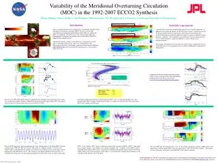
On the path of the Gulf Stream and the Atlantic Meridional Overturning Circulation 1 (AMOC). Terrence Joyce 2 , WHOI Rong Zhang, GFDL. 1 A manuscript of this title was recently published in J. Climate

E N D
On the path of the Gulf Stream and the Atlantic Meridional Overturning Circulation1(AMOC) Terrence Joyce2, WHOI Rong Zhang, GFDL 1A manuscript of this title was recently published in J. Climate 2TJ is solely responsible for preparing this presentation, acknowledges support from PO NASA, & has requested R. Zhang to present this at the US AMOC Science Meeting in June 2010.
Our motivation… • AMOC variability is one of the central diagnostics for understanding global climate change • Until recently with the start of the RAPID moored array at 26N in the Atlantic, we have not been able to readily and accurately measure AMOC change anywhere: repeat hydro sections are too ‘noisy’ • It would be desirable to find a good ‘proxy’ for AMOC change that is readily measurable & can be used for assessing models
Introduction - 1 The Gulf Stream path after it separates from the western boundary near Cape Hatteras tends towards the ENE and is characterized by rings and meanders. The dominant mode of variability, however, is a meridional shift of the entire path between 75 and 55oW. This was first shown in Joyce, Deser and Spall (JCli 2001) using ca. 50 years of subsurface temperature data at 200m oriented along the mean temporal position of the “north wall” of the Gulf Stream. This runs parallel to the large SST gradient seen at the northern side of the warm water in the Gulf Stream in the satellite image at the right.
Introduction - 2 de Coëtlogon et al. (JPO, 2006) examined the GS path variability using our data-based source (upper left), and 5 non-eddy-resolving oceanic general circulation models driven by atmospheric fluxes derived from the NCEP reanalysis. Like the observations, the dominant EOF of path variability (solid lines) from the mean subsurface path based on temperature (dashed lines) was a mean ‘shift’ N/S of the path. While the specific path definition was different in the models the temporal variability of the lowest EOF is similar and significantly correlated with the observed path variability.
Introduction - 3 If the transport from 200:700m depth is regressed against the GS path in each of these models, the northward excursions of the GS path are associated with larger GS flows (variability is in same direction as mean GS). For southward paths, the GS transport in decreased. Significant correlations (90% level) are shown in grey. In each model, the change in the Atlantic Meridional Overturning Circulation (AMOC), defined as the mean annual max of the meridional streamfunction north of 30N, was estimated. Are changes in the AMOC related to the path of the GS?
Introduction - 4 The answer is “yes”, although the relationships are not robust. Time series of the AMOC (solid line) and the GST index (dashed) in the (left) model simulation and (right) observations. Ensemble means are used for MPI-OM and MICOM. The correlation between the two series is indicated. (from de Coëtlogon et al., JPO, 2006). Almost uniformly these models suggest that the AMOC is larger when the GS path is more northward. In our original paper Joyce et al. (2001) we developed a model in which a delayed oscillator dynamics related the strength of the DWBC and the GS at the crossover point near Cape Hatteras. In this model, a stronger DWBC would ‘advect’ the GS offshore leading to a more southerly (not northerly) path.
However, this issue is far from settled… The Principal component time series of the lowest EOF of GS path variability based on altimeter data (north positive, upper), and the PC of the leading EOF of the joint SST and surface geostrophic flow in the Slope Water (positive is colder, more SW’ly flow, middle) are plotted with their lagged correlation. We find significant (at 90% level) correlations indicated as grey dots (lower panel), where significance is based on the observed integral time scales of the two correlated variables. Adapted from Peña-Molino and Joyce (2008). Thus a colder, more SW’ly flow at the surface in the Slope Water leads to a more southerly GS path. Hydro cruises
Line W DWBC moored array A mixed array of Moored Profilers, VACMs, and Seacats has been in the water since 2004, and is ongoing with support from NSF as part of the US AMOC Program.
DWBC composite section along Line W Composite mean section (distance, km, vs. depth, m) across the Line W array starting at 40N, 70W an extending along an altimeter ground track across the bathymetry. Dashed lines in each panel are neutral density surfaces, which are labeled in the third panel. High oxygen and low salinity ‘cores’ demark Labrador Sea Water and GIN Sea Overflow Water (no salinity extremum), that make up North Atlantic Deep Water (NADW), which is found inshore and under the GS on the section. The zero normal velocity contour is in white on the right panel. Adapted from Joyce et al. (2005). We see that an increase in the SW’ly flow at the surface will increase the transport of the DWBC if the change has a depth distribution like the mean flow (right panel).
DWBC and GS path redux • Beatriz Peña-Molino thesis is dealing with Line W data and the relationship between the DWBC variability, Slope Water flow, and the GS path change • Suffice for now in accepting that the velocity variability in the Slope Water is coherent throughout most of the water column and that increases in SW’ly near surface flow are positively correlated with SW’ly transport increases of LSW • The issue of how changes of the DWBC and AMOC are related near 38N is still open: if DWBC and AMOC variability is anti-correlatedor if larger upper level Slope Water flow is associated with a decreased DWBC (and AMOC), there is no inconsistency between the observations and the models • However, the simplest explanation is that the observations are not consistent with the previous model results • Yet consider some new developments…
GFDL CM2.1 coupled climate model study What Zhang (2008) found is that the T400 index (red) constructed from the GFDL CM2.1 1000-year control integration is significantly (at 99% level) correlated (r=0.84) with the AMOC variability (black) at 40N. Therefore, T400 emerges as a “fingerprint” of the AMOC in the coupled model. This result means that a stronger AMOC is associated with a more southerly GS path in the model, also suggested by the recent Line W research, but exactly opposite to the previous modeling work already cited.
The modeling connundrum… • It is unknown why the coupled GFDL model produces a result that is opposite to the previous models • None of these models is eddy-resolving • None of the ‘forced’ ocean models is coupled to the atmosphere – is an active coupling responsible? • It is not clear how well-developed the DWBC is in these forced models – clearly in some, there is no room for a northern re-circulation gyre – the GS is right up against the continental slope. So is a well-established DWBC to north of the GS crossover dynamics necessary? • It is suggested from observations, however, that a stronger DWBC is associated with a more southerly GS path – and this suggests the GFDL model may be ‘correct’ • The latter clearly shows our bias – that models that agree with observations are better than those that don’t!
And a 2nd “observational” result to consider… Balmaseda et al. (GRL, 2007) have made an ocean state estimation (ORA-S3) on a 1x1 deg. grid for the period 1959:2006. In this work, all available subsurface T,S data have been used as well as SST and altimetric data in recent years. Also included since 2003 are Argo profile data. The forcing for this model is the ECMWF ERA40 reanalysis updated using an operational product since 2003. At the right is the time-mean meridional streamfunction of the zonally-integrated AMOC in the upper 3000m of the model (Balmaseda, pers. comm.). Time-varying AMOC will be extracted for the upper 1200m near the max. streamfunction depth.
AMOC and the GS path redux The annual mean (negative) GS index based on T200 and the T400 index from Zhang (2008) are re-plotted with the AMOC index from the Balmaseda et al. calculated near the intergyre boundary (37-38.5N). All indices have recently been updated and corrected for XBT/MBT bias and fall rate errors. While T200 and T400 are significantly correlated (at 95%), the correlations with the AMOC index are marginally correlated in the period of overlap with no lag/leads with the GS path index. One other ocean reanalysis product (GECCO) does not appear to reproduce a correlated signal with the observed GS path.
GS path and T(400m) In the lower panel we show the leading EOF of 50 yr variability of the observed subsurface temperature at 400m (adapted from Zhang, GRL 2008). It is everywhere positive except in the region of the GS. The T400 index (PC1) of this EOF is significantly correlated (r=0.62) at 95% with the negative of the observed GS path index at 200m (upper panel). Input files [WOD9] have corrected MBT/XBT data. From Joyce & Zhang, J. Climate, 2010, 23, 3170–3178. . Tsub EOF1
Summary • AMOC change is one key dynamic examined in virtually all IPCC class models in terms of natural and forced climate variability – its decrease is one key anthropogenic ‘fingerprint’. • Since we do not have a record of the AMOC over the past 50 years, & have only recently begun monitoring at 26N, some useful ‘proxy’ would be desirable. • Various models indicate a significant relationship exists between AMOC variability and the GS path. • However, the sign of this relationship seems to be in serious doubt & more work understanding model response is needed! • Line W observations support models where GS path is southerly(northerly) when the AMOC/DWBC is strong(weak). • This runs against paleo thinking that a more southerly GS was present during the LGM when the AMOC was reduced • GS path is an index which, along with T400, might be compared to various numerical calculations and ocean state estimations regarding AMOC and DWBC variability.