Download
1 / 27
280 likes | 395 Views
Aggregate Expenditure, Equilibrium GDP and The Fiscal policy. The Simple Economy Case. We assume here that we have a simple economy where G = 0 ( no government effect on the economy) and X = 0, M = 0, and hence X-M = 0 (no foreign trade). In such a case the national spending becomes = C + I.

E N D
Aggregate Expenditure, Equilibrium GDP and The Fiscal policy Prof. Abdelhamid Mahboub and Dr. Yousuf Hayajneh
The Simple Economy Case • We assume here that we have a simple economy where G = 0 ( no government effect on the economy) and X = 0, M = 0, and hence X-M = 0 (no foreign trade). • In such a case the national spending becomes = C + I. • Let us start with the consumption spending (expenditure) Prof. Abdelhamid Mahboub and Dr. Yousuf Hayajneh
Consumer Spending and Income • The relationship between the level of income and consumption spending is called the consumption function: Prof. Abdelhamid Mahboub and Dr. Yousuf Hayajneh
Consumer Spending and Income • Ca = autonomous consumption, or the amount of consumption spending that does not depend on the level of income. • by = the part of consumption that is dependent on income, where: • b = marginal propensity to consume (MPC), or the fraction of additional income that is spent. • y = level of income in the economy. Prof. Abdelhamid Mahboub and Dr. Yousuf Hayajneh
The Consumption Function • The consumption function relates desired consumer spending to the level of income. • The consumption function intersects the vertical axis at Ca, the value of autonomous consumption. Prof. Abdelhamid Mahboub and Dr. Yousuf Hayajneh
The Consumption Function • When income equals zero, the value of total consumption (C) equals Ca. It corresponds to the amount of consumption that does not depend on the level of income. Prof. Abdelhamid Mahboub and Dr. Yousuf Hayajneh
The Consumption Function • The slope of the consumption function is the marginal propensity to consume (MPC), or the value of b in the linear equation. Prof. Abdelhamid Mahboub and Dr. Yousuf Hayajneh
Consumer Spending and Income • The fraction that the consumers spend on consumption is given by their MPC. • The fraction that the consumer s save is determined by their marginal propensity to save (MPS). • The sum of the marginal propensity to consume and the marginal propensity to save is always equal to one. MPC + MPS = 1. Prof. Abdelhamid Mahboub and Dr. Yousuf Hayajneh
Changes in the Consumption Function • The consumption function can change for two reasons: • A change in autonomous consumption. • A change in the marginal propensity to consume. Prof. Abdelhamid Mahboub and Dr. Yousuf Hayajneh
Changes in the Consumption Function • Factors that cause autonomous consumption to change are: • Consumer wealth, or the value of stocks, bonds, and consumer durables held by the public (i.e. the consumers). More wealth => higher consumption spending. • Consumer confidence. More confidence => higher consumption spending. Prof. Abdelhamid Mahboub and Dr. Yousuf Hayajneh
Changes in the Consumption Function • An increase in autonomous consumption from C0a to C1a shifts up the entire consumption function. Prof. Abdelhamid Mahboub and Dr. Yousuf Hayajneh
Changes in the Consumption Function • An increase in the MPC from b to b’ increases the slope of the consumption function. Prof. Abdelhamid Mahboub and Dr. Yousuf Hayajneh
Changes in the Consumption Function • The consumption function is determined by the level of autonomous consumption and by the MPC. Prof. Abdelhamid Mahboub and Dr. Yousuf Hayajneh
Changes in the Consumption Function • Factors that cause the marginal propensity to consume to change are: • Perception of changes in income. Studies show that consumers tend to save a higher proportion of a temporary increase in income, and spend a higher proportion if the increase is perceived to be permanent. • Changes in taxes. Prof. Abdelhamid Mahboub and Dr. Yousuf Hayajneh
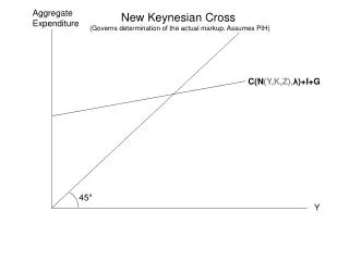
Determining GDP • GDP is determined where the C + I line intersects the 45 line. • At that level of output, y*, desired spending equals output. Prof. Abdelhamid Mahboub and Dr. Yousuf Hayajneh
Savings and Investment • Savings equals output minus consumption. • Output is determined by demand, C + I, or • Subtracting consumption from both sides of the equation results in: • The left side shows that y – C equals savings, S, therefore: Prof. Abdelhamid Mahboub and Dr. Yousuf Hayajneh
Savings and Investment • Equilibrium output is determined at the level of income where savings equals investment: • The level of savings in the economy is not fixed, and how it changes depends on the real GDP. • The savings function is the relationship between the level of income and the level of savings. Prof. Abdelhamid Mahboub and Dr. Yousuf Hayajneh
The Multiplier • The multiplier is the ratio of the change in equilibrium output to the change in spending. It measures the degree to which changes in spending are “multiplied” into changes in output. Prof. Abdelhamid Mahboub and Dr. Yousuf Hayajneh
The Multiplier • An increase in investment shifts the C + I line upward. • When investment increases by ΔI from I0 to I1, equilibrium output rises by Δ y from y0 to y1. Prof. Abdelhamid Mahboub and Dr. Yousuf Hayajneh
The Multiplier • The change in equilibrium output (Δy) is greater than the change in investment (ΔI). • The value of the multiplier = 1/(1-b) • 1/(1-b) > 1. Why? Prof. Abdelhamid Mahboub and Dr. Yousuf Hayajneh
The Multiplier in Action (if b = 0.8) Prof. Abdelhamid Mahboub and Dr. Yousuf Hayajneh
The Multiplier in Action (if b = 0.8) • In this numerical example notice that The value of the multiplier = 1 / (1-b) = 1 / (1-0.8) = 1 / 0.2 = 5 • And Δ y = ΔI × the multiplier = 10 × 5 = 50 Prof. Abdelhamid Mahboub and Dr. Yousuf Hayajneh
The Multiplier in Action • In general: The final change in equilibrium output or income = the initial change in spending × the multiplier. • The change could be an increase or a decrease. • The source of the change in spending could be from consumption or investment or any other source of expenditure. Prof. Abdelhamid Mahboub and Dr. Yousuf Hayajneh
The Fiscal Policy • More realistically, we should include in our model the two other items of spending (expenditure) that we assumed out before. • Therefore, AE = C + I + G + (X – M) • AE will change when one or more of its components (on the right hand side) change. • An intentional government action to change AE is called “government economic policy” or “government policy” for short. Prof. Abdelhamid Mahboub and Dr. Yousuf Hayajneh
The Fiscal Policy • The “fiscal policy” refers to one type of the government policy actions to change the level of GDP through changing the government expenditure or taxes. • Recall that AE = C + I + G + (X – M), and therefore if the government changes its expenditure while all other things remain constant we will have Δ AE = Δ G. • Increasing (decreasing) G by 1 billion SR leads to an equal increase (decrease) in AE. Prof. Abdelhamid Mahboub and Dr. Yousuf Hayajneh
The Fiscal Policy • If the government knows that the value of expenditure multiplier = 5 and it increases its expenditure by 1 billion SR, it should expect an increase in GDP by 5 billion SR. We refer here to the formula on slide no. 24 before. • If reducing taxes leads to an increase in C by 1 billion SR, we expect the same effect. • Notice that the final increase in GDP will take some time to appear. This time length varies from one economy to another. Prof. Abdelhamid Mahboub and Dr. Yousuf Hayajneh
Test yourself • Why do we say MPC + MPS = 1? Is it possible to be greater than 1? Why or why not? • If MPC = 0.75 and the government raised G by 40 million SR, what do you expect to happen to GDP? • Give a definition of MPC, MPS and the multiplier. • The value of the expenditure multiplier can not be less than 1. Why is this true? • If MPC = 0.8 and we need GDP to increase by 10 billion SR, what can the fiscal policy do in order to achieve this goal? Prof. Abdelhamid Mahboub and Dr. Yousuf Hayajneh