Download
1 / 44
450 likes | 712 Views
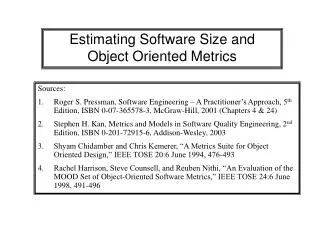
Estimating Software Size and Object Oriented Metrics. Sources: Roger S. Pressman, Software Engineering – A Practitioner’s Approach, 5 th Edition, ISBN 0-07-365578-3, McGraw-Hill, 2001 (Chapters 4 & 24)

E N D
Estimating Software Size and Object Oriented Metrics • Sources: • Roger S. Pressman, Software Engineering – A Practitioner’s Approach, 5th Edition, ISBN 0-07-365578-3, McGraw-Hill, 2001 (Chapters 4 & 24) • Stephen H. Kan, Metrics and Models in Software Quality Engineering, 2nd Edition, ISBN 0-201-72915-6, Addison-Wesley, 2003 • Shyam Chidamber and Chris Kemerer, “A Metrics Suite for Object Oriented Design,” IEEE TOSE 20:6 June 1994, 476-493 • Rachel Harrison, Steve Counsell, and Reuben Nithi, “An Evaluation of the MOOD Set of Object-Oriented Software Metrics,” IEEE TOSE 24:6 June 1998, 491-496
A Good Manager Measures process process metrics project metrics measurement product metrics product What do we use as a basis? • size? • function?
Why do we Measure? • To characterize – to gain understanding of process, products, resources, and environments, and to establish baselines for future assessments • To evaluate – to determine status with respect to plans. • To predict – so that we can plan. • To improve – we gather information to help us identify road blocks, root causes, inefficiencies, and other opportunities for improving product quality and process performance.
Product Metrics • focus on the quality of deliverables • measures of analysis model • complexity of the design • internal algorithmic complexity • architectural complexity • data flow complexity • code measures (e.g., Halstead) • measures of process effectiveness • e.g., defect removal efficiency
UML-Based Sizing and Use Case Points • One approach to software sizing is to use the products of analysis as a basis for early reliable measures of size. This is called “process estimation.) • Though requirements are still a crude way to quantify the functionality of a software product, UML provides a standard notation, and it is considered an industry standard. • A use case is one of the components of UML. Use cases do not capture nonfunctional requirements nor are they simply a functional decomposition of the system. • Use cases capture functions and data in user terms. • Use case points (UCPs) are metric to estimate effort for projects [Gustav Karner, 1993].
Steps to Count Use Case Points • Identify the actors and assign a weight based on how they interact with the system of interest: 2. Sum the weights for the actors in all use cases to obtain the unadjusted actor weight, UAW
3. Identify use cases, and assign a complexity to each use case based on the number of transactions or scenarios that each use case contains: Alternatively, you can use “analysis classes” to estimate the use case complexity. I prefer this method because it less subjective. • Sum the weight for all the use cases to obtain the unadjusted use weight, UUCW. • Sum UAW and UUCW to obtain the size in unadjusted use case points (UUCPs).
Adjust for the technical complexity of the product by rating the degree of influence of each of the 13 factors. The ratings range from 0 to 5; 0 means that the factor is irrelevant for the project; 5 means that it is essential. The 13 factors and their associated weights are:
For each factor, multiply the degree of influence by the weight, and sum the products to obtain the technology sum, TSUM. Use the weights table shown in the table in the preceding step. • Compute the technical complexity factor, TCF, using TCF = 0.6 + 0.01 * TSUM • Adjust for the “envirenment,” which addresses the skills and training of the staff, precedentedness, and requirements stability. There are eight factors:
Rate each factor’s influence from 0 to 5, with 3 denoting “average.” For factors F1 through F4, 0 means no experience in that area, and 5 means expert. For factor F5, 0 means no motivation, and 5 means high motivation. For factor 6, 0 means extremely unstable requirements and 5 means unchanging requirements. For factor F7, 0 means no part-time staff, and 5 means all part-time staff. For factor F8, 0 means an easy-to-use programming language, and 5 means a very difficult programming language. • For each factor, multiply the degree of influence by the weight, and sum the products to obtain the environment sum ESUM • Compute the environment factor, EF, using EF = 1.4 – 0.03*ESUM • Compute the size in (adjusted) Use Case Points (UCPs) using UCP = UUCP * TCF * EF
Function Points • Function points [Allan J. Albrecht, 1979] are a software size measure designed to meet three goals: • Gauge delivered functionality in terms users can understand • Be independent of technique, technology, and programming language • Give a reliable indication of software size during early design
The Counting Rules • Function point analysis (FPA) quantifies product functionality in terms of five externally visible system elements, called function types, that are readily understood by both users and developers: • EI: External input – is a related group of user data or control information that enters the boundary of the application and adds or changes data in an internal logical file, or used to perform some function or calculation.
EO: External output – is a related group of user data or control information that leaves the boundary of the application. • EQ: External query – is a related group of user data or control information that enters the boundary of the application and generates an immediate output of a related group of user data or control information. A query is a set of selection criteria that are used to extract information from an existing database. • ILF: Internal logical file – is a user identifiable group of logically related data or control information that (i) resides within the boundary of the application, and (ii) is maintained and used by the application. • EIF: External interface file – is a user-identifiable group of logically related data or control information that (i) resides outside of the application boundary, and (ii) is used by the application for some of its processing. • Function point counting is a type of Linear Method.
Weights for Function Points and Feature Points • Feature points [Capers Jones, 1985] is a simplified size measure compared to function points. • Feature point also identifies a sixth data type, algorithms, to account for complex calculation.
For each function type and complexity, the count is multiplied by the corresponding weight. • Summing the results for all 15 pairs (5 function types and 3 complexity levels) gives the total number of unadjusted function points (UFPs) for the software product. • This total (UFPs) is adjusted for the general system characteristics (GSCs) of the product. • Table (next slide) lists the 14 GSCs and some of the main factors considered in assigning a value. • Each factor is rated based on its “degree of influence” (0 = no influence, up to 5 = strong influence). • Summing these 14 ratings gives the total degree of influence (TD1) which is used to compute value adjustment factor (VAF), as follows: • TDI = 14j=1Rating and VAF = 0.65 + 0.01*TDI
Applying the value adjustment factor gives the software size in adjusted function points (AFPs): Size(AFPs) = VAF*Size(UFP) • The VAF can increase or decrease the size by no more than 35%. • The “dynamic range” of the size adjustment is 2 (=1.35/0.65)
Advantages and Disadvantages of Function-Based Sizing • It facilitates the dialogue between the user of the system and the developer. • FP estimates are generally claimed to be accurate within 10% • FP counting cannot take place until the requirements are reasonably well understood and the high level design of the system is known. • A main disadvantage of FPs is that they must be counted manually. This is expensive. • FP only gives the (functional) size of a software not the estimate development effort or time. • Other concerns with functional size measurement [Norman Fenton and Shari Pfleeger] are given in the table below.
Defining Source Lines of Code (SLOC) • Code may originate from different sources as shown below and this must be considered when counting SLOC
The following table provides rough estimates of the average number of lines of code required to build one function point in various programming languages: Programming LanguageLOC/FP (average) Assembly language 320 C 128 COBOL 106 FORTRAN 106 Pascal 90 C++ 64 Ada95 53 Visual Basic 32 Smalltalk 22 Powerbuilder (code generator) 16 SQL 12
The Constructive Cost Model (COCOMO • COCOMO is the classic LOC cost-estimation formula. • It was created by Barry Boehm in the 1970s • He used thousand delivered source instructions (KDSI) as his unit of size. KLOC is equivalent. • His unit of effort is the programmer-month (PM). • Boehm divided the historical project data into three types of projects: • Application (separate, organic, e.g., data processing, scientific) • Utility programs (semidetached, e.g., compilers, linkers, analyzers) • System programs (embedded)
He determined the values of the parameters for the cost model for determining effort: • Application programs: PM = 2.4*(KDSI)1.05 • Utility programs: PM = 3.0*(KDSI)1.12 • Systems programs: PM = 3.6*(KDSI)1.20 • Boehm also determined development time (TDEV) in programmer-months: • Application programs: TDEV = 2.5*(PM)0.38 • Utility programs: TDEV = 2.5*(PM)0.35 • Systems programs: TDEV = 2.5*(PM)0.32
The CAD software will accept two- and three-dimensional geometric data from an engineer. The engineer will interact and control the CAD system through a user interface that will exhibit characteristics of good human/machine interface design. All geometric data and other supporting information will be maintained in a CAD database. Design analysis modules will be developed to produce the required output, which will be displayed on a variety of graphics devices. The software will be designed to control and interact with peripheral devices that include a mouse, digitizer, laser printer, and plotter. Compute LOC/FP using estimates of information domain values Use historical effort for the project For our purposes, we assume that further refinement has occurred and that the following major software functions are identified: User interface and control facilities (UICF) Two-dimensional geometric analysis (2DGA) Three-dimensional geometric analysis (3DGA) Database management (DBM) Computer graphics display facilities (CGDF) Peripheral control function (PCF) Design analysis modules (DAM) Conventional Methods: LOC/FP Approach
Object Oriented Measurement • The measurement of object-oriented software has the same goals as the measurement of conventional software – trying to understand the characteristics of the software. • Traditional software measurement uses control flow graph as the basic abstraction of the software. The control flow graph does not appear to be useful as an abstraction of object-oriented software. • The intuitive problem with applying the traditional software metrics is that the complexity of object-oriented software does not appear to be in the control structure. • In most object-oriented software, the complexity appears to be in the calling patterns among the methods.
Weighted Methods per Class (WMC) • The WMC metric is based on the intuition that the number of methods per class is a significant indication of the complexity of the software. • Let C be a set of classes each with the number of methods M1, ..., Mn. Let c1, ..., cn be the complexity (weights) of the classes (assume ci is equal to 1). • This is the only metric that is averaged over the classes in a system
Depth of Inheritance Tree (DIT) • The depth of inheritance tree metric is just the maximum length from any node to the root of the inheritance tree for that class. • Inheritance can add to complexity of software. This metric is calculated for each class. Number of Children (NOC) • Not only is the depth of the inheritance tree significant, but the width of the inheritance tree. • The number of children metric is the number of immediate sub-classes subordinated to a class in the inheritance hierarchy. This metric is calculated for each class.
Coupling between Object Classes (CBO) • In object-oriented, coupling can be defined as the use of methods or attributes in another class. • Two classes will be considered coupled when methods declared in one class use methods or instance variables defined by the other class. • Coupling is symmetric. If class A is coupled to class B, then B is coupled to A. • The coupling between object classes (CBO) metric will be the count of the number of other classes to which it is coupled. • This metric is calculated for each class.
Response For a Class (RFC) • The response set of a class, {RS}, is the set of methods that can potentially be executed in response to a message received by an object of that class. • It is the union of all methods in the class and all methods called by methods in the class. • It is only counted on one level of call. RFC = |RS| • The metric is calculated for each class
Lack of Cohesion in Methods (LCOM) • A module (or class) is cohesive if everything is closely related. The lack of cohesion in methods metric tries to measure the lack of cohesiveness. Let Ii be the set of instance variables used by method I. Let P be set of pairwise null intersections of Ii. Let Q be set of pairwise nonnull intersections. • LCOM metric can be visualize by considering a bipartite graph. One set of nodes consists of attributes, and the other set of nodes consists of the functions. An attribute is linked to a function if that function accesses or sets that attributes. • The set of arcs is the set Q. If there are n attributes and m functions, then there are a possible n * m arcs. So, the size of P is n + m minus the size of Q. LCOM = max(|P| - |Q|, 0) • This metric is calculated on a class basis.
The MOOD (Metrics for Object Oriented Design) The MOOD suite of metrics is intended as a complete set that measures the attributes of encapsulation, inheritance, coupling, and polymorphism of a system. • Let TC be the total number of classes in the system. • Let Md(Ci) be the number of methods declared in a class i. • Consider the predicate Is_visible(Mm,i, Cj), where Mm,i is the method m in class i and Cj is the class j. This predicate is 1 if i != j and Cj may call Mm,i. Otherwise, the predicate is 0. For example, a pubic method in C++ is visible to all other classes. A private method in C++ is not visible to other classes. The visibility, V(Mm,i), of a method, Mm,i is defined as follows:
Encapsulation – MHF and AHF • The method hiding factor (MHF) and the attribute hiding factor (AHF) attempt to measure the encapsulation. • Where Ad(Ci) is the number of attributes declared in a class and • V(Am,i) is the visibility of an attribute, Am,i
Inheritance Factor – MIF and AIF • There are two measures of the inheritance, the method inheritance factor (MIF) and the attribute inheritance factor (AIF). Let Md(Ci) be the number of methods declared in a class i Let Mi(Ci) be the number of methods inherited (and not overridden) in a class i Let Ma(Ci) = Md(Ci) + Mi(Ci) = Number of methods that can be invoked in association with class i
Inheritance Factor – MIF and AIF cont.. Let Ad(Ci) = Number of attributes declared in a class i Let Ai(Ci) = Number of attributes from base classes that are accessible in a class i Let Aa(Ci) = Ad(Ci) + Ai(Ci) = Number of attributes that can be accessed in association with class i
Coupling Factor (CF) • The coupling factor (CF) measures the coupling between classes excluding coupling due to inheritance. • Let is_client(Ci, Cj) = 1 if class i has a relation with class j; otherwise, it is zero. • The relationship might be that class i calls a method in class j or has a reference to class j or to an attribute in class j. • This relationship cannot be inheritance.
Example 3 – Calculate the coupling factor on the object model shown below for B & B problem. Only assume a relationship if it is required by the association shown on the diagram
Polymorphism Factor (PF) • The polymorphism factor (PF) is a measure of the potential for polymorphism. • Let Mo(Ci) be the number of overriding methods in class i. • Let Mn(Ci) be the number of new methods in class i. • Let DC(Ci) be the number of descendants of class i.
Example 4 – Calculate the polymorphism factor on the C++ code from example 2 above: