Download
1 / 23
230 likes | 387 Views
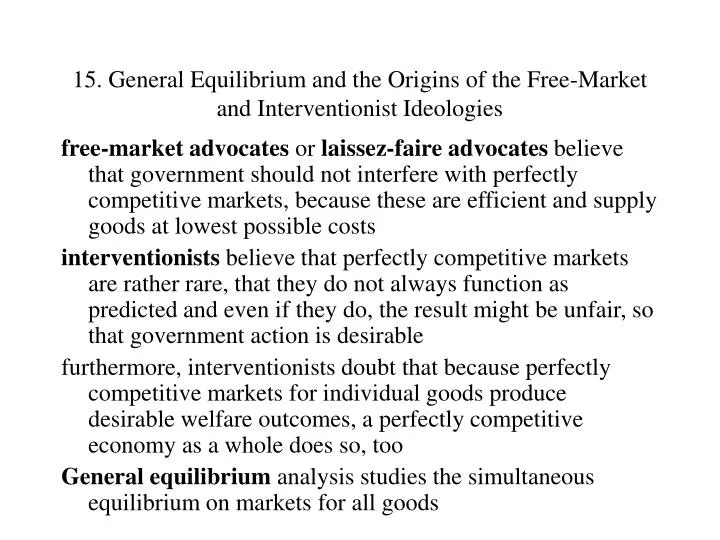
15. General Equilibrium and the Origins of the Free-Market and Interventionist Ideologies. free-market advocates or laissez-faire advocates believe that government should not interfere with perfectly competitive markets, because these are efficient and supply goods at lowest possible costs

E N D
15. General Equilibrium and the Origins of the Free-Market and Interventionist Ideologies free-market advocates or laissez-faire advocates believe that government should not interfere with perfectly competitive markets, because these are efficient and supply goods at lowest possible costs interventionists believe that perfectly competitive markets are rather rare, that they do not always function as predicted and even if they do, the result might be unfair, so that government action is desirable furthermore, interventionists doubt that because perfectly competitive markets for individual goods produce desirable welfare outcomes, a perfectly competitive economy as a whole does so, too General equilibrium analysis studies the simultaneous equilibrium on markets for all goods
15.1 The Free-Market Argument basic assumptions: • existing economy with given stock of capital and labor • large number of people who are both consumers and producers • consumers have convex preferences, producers convex technology • for illustration 2 goods, 2 people: one produces good 1, the other good 2 aim: allocate inputs efficiently in production, distribute goods efficiently to consumers (Pareto-efficiency) free-market argument: beliefs: • perfect competition leads to efficient allocation of inputs • competitive markets lead to efficient distribution of goods once they are produced • the final product mix is determined by the income distribution that results from competitive market
Efficiency in Consumption given some output of the economy, the goods are efficiently distributed if the marginal rate of substitution between each pair of goods is the same for all consumers, allocation must lie on the contract curve otherwise if, e.g. two consumers have MRS 1/4 and 1/2, they can both be better off by trading at a rate 1/3 Efficiency in Production efficient allocation of inputs can be studied analogously: in an Edgeworth box with dimension given by the existing labor force and capital stock, inputs spent on good 1 are measured from origin, on good 2 from upper right when isoquants cross, there are other allocations of inputs that yield more of both goods (Fig 15.2) hence in efficient allocation isoquants have to be tangent and therefore, the marginal rates of technical substitution have to be equal for all goods; otherwise relative productivity of one factor is higher for one good than for another good
Consistency of Production and Consumption the various efficient allocations of inputs yield the production possibilities frontier that describes all combinations of goods that can be produced efficiently (Fig 15.3) its slope indicates how many units of good 2 have to be given up for an additional unit of good 1, the marginal rate of transformation (MRT) we have MRT2 for 1 = MC1 / MC2 a given product bundle on the frontier now spans an Edgeworth box, the points in it represent the possible allocations of goods (Fig 15.4) production and consumption are consistent for a point on the contract curve where MRT = MRS for all consumers otherwise, if e.g. MRS > MRT there is another efficient product mix (more of good 1 and less of good 2) that will make all consumers and producers better off
Perfectly Competitive Markets Satisfy the Conditions for Pareto Efficiency Efficiency in Consumption: in perfectly competitive market, all consumers can buy as much as they want at identical prices; they buy a combination such that MRS2 for 1 = p1/p2; since all consumers do the same, all MRS are equal Efficiency in Production: if factor markets are perfectly competitive, firms can buy inputs at identical costs; they will use input combination such that MRTSc for l = wl / wc; since all firms do the same, all MRTS will be equal Consistency of Production and Consumption: in a long-run equilibrium, prices equal marginal costs, hence p1/p2=MC1/MC2. Since all consumers buy a combination such that MRS2 for 1 = p1/p2 =MC1/MC2 and MC1/MC2=MRT2 for 1, we get MRS2 for 1 = MRT2 for 1, as required
The Two Fundamental Theorems of Welfare Economics first fundamental theorem of welfare economics: every competitive equilibrium is a Pareto-optimal equilibrium for the economy second fundamental theorem of welfare economics: every Pareto-optimal allocation can be achieved as a competitive equilibrium for an appropriate distribution of income hence if one wants to reach a specific Pareto-optimal outcome, only redistribution of income is necessary, but not intervention in the price mechanism of the markets thus if one considers Pareto-optimality as desirable, government intervention should be reduced to income redistribution
15.2 The Interventionist Argument basic concern: not only Pareto-optimality should be considered, but also equity in a perfectly competitive economy, for each point on the production possibility frontier, a Pareto-optimal distribution will be reached (Fig 15.5) different product mixes lead to different utility combinations utilities possibilities frontier marks the maximal achievable utility combinations the product mix that is chosen depends on the distribution of wealth and labor (i.e. the individual productivity of labor) interventionists believe that endowments should not determine the utility hence government should intervene to reach more equitable level, even though this might not be Pareto-efficient
A Basis for Intervention: Rawlsian Justice Rawls’ Maximin Justice: the welfare of the least well-off person should be maximized Justification: assume people decide upon distribution under a “veil of ignorance”, i.e. they do not know their position in society under such a veil of ignorance, they would probably agree to a distribution that maximizes well-being of the least well-off person, because they might be that person hence increasing inequality can be acceptable if the least well-off person is made better off (e.g. if tax cuts for the rich lead to more and better paid jobs for the poor)
A Free-Market Rebuttal to Rawls: Nozick’s Process Justice Process Justice: if an outcome is reached by voluntary agreements of all people involved, it is justified Problem: if the initial distribution of wealth is very unequal, even if all agents act voluntarily, it may stay unequal counter-argument (from a moderate free-market advocate): if one wants to rectify inequality, one should then redistribute income before market process starts, but not interfere with the market process Equitable Income Distribution: Varian’s Envy-Free Justice envy-free allocation: nobody prefers another agent’s bundle over their own envy-free allocation will be reached when all start with identical bundles and trade at competitive prices; no agent will envy another because he could have had his bundle unequal distribution can be just when it is envy-free Problems: utility levels can still differ, envy-freeness does not imply Pareto-efficiency and vice versa
15.3 Institutional Failure: Another Interventionist Argument institutions have developed to solve a multitude of problems: perfectly competitive markets for exchange, insurance to cover risks, regulatory agencies to deal with monopolies a competitive market solves a problem efficiently; so if one wants to reach efficiency, a problem that can be solved by a competitive market should be left to a market without intervention however, if problems include asymmetric information, public goods, externalities, moral hazard and incomplete information, markets do not work properly in these situations, markets do not only fail to reach equity but also efficiency non-market institutions may develop to solve the problem, but they do not necessarily work efficiently either if also non-market institutions fail, intervention may be necessary
19. Input Markets and the Origins of Class Conflict capital and labor are unevenly distributed, so income will be unequal as well this creates the potential for conflicts about the appropriate returns to the different factors 19.1 Why It Is Important to Determine the Return on Each Factor of Production apparently market economies are more efficient than central planning economies, but this does not mean that everybody is happy with the return on the factor they provide the division into workers, capitalists, and landowners provides a source of conflict the question is whether the returns are fair and reasonable hence we have to study how these returns are determined in competitive and noncompetitive markets
19.2 The Return on Labor In an competitive market, the return on labor is determined by the supply and demand a firm’s demand for labor is determined by its desire to maximize profit, hence it is a derived demand the output due to an additional unit of labor is the marginal physical product; due to diminishing returns to each factor, the MPP is decreasing (Fig 19.1) a profit-maximizing firm is interested in the increase of revenue an additional unit of labor yields, the marginal revenue product which is the MPP times the marginal revenue that the output yields, hence MRP = MR * MPP in perfectly competitive industry, MR = p, MRP = p * MPP for a monopolist, the MR is falling, so the MRP curve is steeper than for a competitive firm (but the MR may initially be higher than p in a competitive market, so monopolist’s MRP does not have to be below competitive MRP everywhere) (Fig 19.2)
the optimal quantity of labor is the one where the MRP is equal to the MC of labor given a perfectly competitive labor market, the MC is constant, the firm faces a constant market wage since a monopolist reduces output, its labor demand will be smaller than that of a competitive firm (more precisely, than that of a competitive industry) (Fig 19.3) a firm’s labor demand curve equals its MRP curve the market demand curve is given as usual by adding individual firms’ demand curves horizontally individual workers decide for each wage how much labor they want to supply by choosing optimal trade-off between leisure and consumption (this is likely to be increasing in some range, but not necessarily throughout, e.g. problem 19.2, labor supply is independent of wage) market supply curve is again horizontal sum equilibrium market wage is determined by supply = demand
19.3 Setting the Stage for Class Conflict given the market equilibrium wage w, a firm will hire labor up to the point where w = MRP (Fig 19.9) since the MRP is falling, the firm hence makes a surplus; workers may demand a share of this surplus, firm argues that surplus is needed for return on capital and land 19.4 The Return on Capital capital consists of manufactured inputs, opposed to naturally occurring inputs labor and land building capital requires money, either borrowed or own costs are interest or opportunity cost of foregone interest if entrepreneurs need money for investments and others have savings to invest, institution is needed to match them financial markets develop how is the market interest rate determined?
The Supply of Loanable Funds given a interest rate, a consumer can trade off consumption today and consumption tomorrow (Fig 19.10) for a sufficiently high interest rate the consumer would be willing to safe today to consume more tomorrow the optimal savings decision is such that MRStomorrow vs today = 1 + r, r = interest rate if consumption tomorrow is a superior good, then higher interest rate implies more consumption tomorrow (but NOT necessarily less consumption today, i.e. higher savings) if higher interest imply higher savings, the supply of loanable funds is upward sloping (Figs 19.11, 19.12) market supply is derived as usually by adding horizontally
The Demand for Loanable Funds an entrepreneur will take a loan and invest it if the expected rate of return of the investment is higher than the interest rate if an investment of C yields R in one period and C(1+) = R, then is the rate of return for a long term investment of C that yields Rk in period k, the rate of return is given by such that C = k Rk / (1+)k for a lower market interest rate more investment projects will be executed; hence the demand curve is downward sloping market demand is again the horizontal sum in market equilibrium supply = demand and the market interest rate equals the marginal rate of return
19.5 The Return on Land a rent is the return on a factor in excess of the amount necessary to ensure that it will be supplied the supply of land is fixed, hence the same amount will be supplied at any return and hence the whole return is a rent the return will be determined by the demand alone (Fig 19.16) 19.6 Resolving the Claims of Different Factors of Production: The Product Exhaustion Theorem marginal productivity theory: each factor is paid its marginal contribution, i.e. labor is paid the MRP of the last worker, capital is paid the rate of return of the last unit a theory of income distribution should predict that the whole value of the goods produced will be distributed
product exhaustion theorem predicts this: in long-run equilibrium, when all factors are paid their marginal revenue product, the sum equals the total value let x1,...,xn be the factors, and w1,...,wn be the prices and y be the quantity of output produced, then in competitive markets all factors are paid their MRP, so requirement is py = w1x1 +...+ wnxn or p = (w1x1 +...+ wnxn) / y this means the price of the good should equal the long-run average cost, but this holds in long-run equilibrium of a perfectly competitive market however, workers could argue that they want a higher wage at the expense of the return on land, because the supply of land would not be reduced
19.7 Determining the Return on Labor in Markets That Are Less Than Perfectly Competitive labor markets can be less than perfectly competitive: a union that encompasses all workers in an industry is a monopolist, a factory in a small town with no other major employers is essentially a monopsonist, the only buyer an employer in a perfectly competitive labor market faces an infinitely elastic supply curve and cannot affect wages an employer who has a monopsony faces an upward-sloping supply curve and hence has a choice about the wage level if the monopsonist cannot apply wage discrimination, i.e. has to pay the same wage to all workers, there is an incentive to lower the demand to reduce the wage: the marginal expenditure (ME) is the increase of total wage due to hiring one more worker ME =w in perfectly competitive market, but for monopsonist ME = w + (dw/dL) L and hence ME is above supply curve
in a perfectly competitive market, the equilibrium would be where marginal revenue product = supply (Fig 19.17) a monopolist will hire labor up to the point where MRP=ME the wage that he offers is given on the supply curve for that employment level MRP = ME = w+(dw/dL)L=w [1+(dw/dL) (L/w)] = w (1+1/) where being the elasticity of labor supply rearranging yields (MRP – w) / w = 1 / hence the less elastic the labor supply, the more is labor paid below its marginal revenue product, or the stronger is the monopsonistic exploitation
in a bilateral monopoly there is only one buyer and one seller, e.g. only one employer and one labor union where all workers are organized we cannot follow the approach of monopoly and monopsony to treat one side of the market as price takers and let the other optimize: unionized workers will not simply accept a monopsonistic wage; monopsonist will not simply accept a monopoly wage set by the union if the union treats the monopsonist as a price taker, i.e. assumes that the demand is given by the MRP curve, the union will choose a quantity such that its marginal revenue (<demand) equals the marginal cost (Fig 19.18) hence both with monopsonist and with monopolistic union, the amount of labor would be below equilibrium in bilateral monopoly, no side is a price taker; the wage depends on the bargaining power of firm and union
The Alternating Offer Sequential Bargaining Institution as a Stylized Model of Bargaining in Bilateral Monopoly • time is divided in discrete periods (say here 3 periods) • the pie to be split shrinks from period to period • in period 1, player A (say the employer) makes a proposal • if B (the union) accepts, the proposal is implemented and the game ends • if B rejects, period 2 starts: the pie shrinks and B makes a proposal • if A accepts, B’s proposal is implemented and the game ends • if A rejects, in period 3 the pie shrinks and A makes a new proposal • if B accepts, the proposal is implemented, if B rejects, both get 0, the game is over a game with more than 3 periods just continues in the same way
theorem: there is a unique subgame perfect equilibrium, where the first offer is accepted and each player obtains the sum of the decrements of the pie when his or her offers are rejected proof: backward induction: in the last period n the player who makes the offer (E) obtains the whole pie x (-) hence in period n-1, player D has to offer E exactly x (E would reject any lower offer) but that means if in period n-1 the pie is y, D suggests to keep y-x for himself hence in period n-2, E has to offer D y-x so if in period n-2 the pie is z, E can suggest to keep z-(y-x)= (z-y)+x which is the sum of the decrements of the pie in periods n and n-2, where E chooses by repeated application of the same argument we see that both players get the total amount by which the pie decreases if their respective offers are rejected experimental evidence: subjects do one period b.i., not more